12 Global Search Methods
As previously mentioned in Chapter 10, global search methods investigate a diverse potential set of solutions. In this chapter, two methods (genetic algorithms and simulated annealing) will be discussed in the context of selecting appropriate subsets of features. There are a variety of other global search methods that can also be used, such as particle swarm optimization and simultaneous perturbation stochastic approximation. Spall (2005) and Weise (2011) are comprehensive resources for these types of optimization techniques.
Before proceeding, the naive Bayes classification model will be discussed. This classifier will be used throughout this chapter to demonstrate the global search methodologies.
12.1 Naive Bayes Models
To illustrate the methods used in this chapter, the OkCupid data will be used in conjunction with the naive Bayes classification model. The naive Bayes model is computationally efficient and is an effective model for illustrating global search methods. This model uses Bayes formula to predict classification probabilities.
\[ \begin{align} Pr[Class|Predictors] &= \frac{Pr[Class]\times Pr[Predictors|Class]}{Pr[Predictors]} \notag \\ &= \frac{Prior\:\times\:Likelihood}{Evidence} \notag \end{align} \]
In English:
Given our predictor data, what is the probability of each class?
There are three elements to this equation. The prior is the general probability of each class (e.g., the rate of STEM profiles) that can either be estimated from the training data or determined using expert knowledge. The likelihood measures the relative probability of the observed predictor data occurring for each class. And the evidence is a normalization factor that can be computed from the prior and likelihood. Most of the computations occur when determining the likelihood. For example, if there are multiple numeric predictors, a multivariate probability distribution can be used for the computations. However, this is very difficult to compute outside of a low-dimensional normal distribution or may require an abundance of training set data. The determination of the likelihood becomes even more complex when the features are a combination of numeric and continuous values. The naive aspect of this model is due to a very stringent assumption: the predictors are assumed to be independent. This enables the joint likelihood to be computed as a product of individual statistics for each predictor.
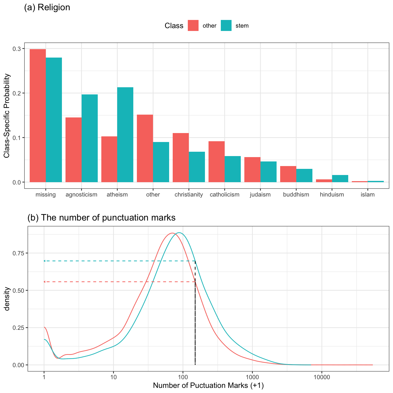
For example, suppose a naive Bayes model with two predictors: the number of punctuation marks in the essays as well as the stated religion. To start, consider the religion predictor (which has 10 possible values). For this predictor, a cross-tabulation is made between the values and the outcome and the probability of each religion value, within each class, is computed. Figure 12.1(a) shows the class-specific probabilities. Suppose an individual listed their religion as atheist. The computed probability of being an atheist is 0.213 for STEM profiles and 0.103 otherwise.
For the continuous predictor, the number of punctuation marks, the distribution of the predictor is computed separately for each class. One way to accomplish this is by binning the predictor and using the histogram frequencies to estimate the probabilities. A better approach is to compute a nonparametric density function on these data (Wand and Jones 1994). Figure 12.1(b) shows the two density curves for each class (with a \(\log_{10}\) transformation on the predictor data). There is a slight trend where the non-STEM profiles trend to use less punctuation. Suppose that an individual used about 150 punctuation marks in their essay (indicated by the horizontal black line). To compute the relative density for each class, the corresponding heights of the density lines for each class are used. Here, the density for a STEM profile was 0.697 and was 0.558 for non-STEMs.
Now that the statistics have been calculated for each predictor and class value, the overall prediction can be made. First, the values for both predictors are multiplied together to form the likelihood statistic for each class. Table 12.1 shows the details for the computations. Both religion and the punctuation mark data were more consistent with the profile being STEM; the ratio of likelihood values for the classes is \(0.148 \div 0.057 = 2.59\), indicating that the profile is more likely to correspond to a STEM career (based on the training data). However, Bayes’ Rule also includes a term for the prior information, which is the overall rate that we would find STEM profiles in the population of interest1. In these data, the STEM rate was about 18.5%, which is most likely higher than in other parts of the country. To get the final prediction, the prior and likelihood are multiplied together and their values are normalized to sum to one to give us the posterior probabilities (which are just the class probability predictions). In the end, the probability that this particular profile is associated with a STEM job is only 37%; our prior information about the outcome was extreme enough to contradict what the observed data were indicating.
| Class |
Predictor Values
|
Likelihood | Prior | Posterior | |
|---|---|---|---|---|---|
| Religion | Punctuation | ||||
| STEM | 0.213 | 0.697 | 0.148 | 0.185 | 0.370 |
| other | 0.103 | 0.558 | 0.057 | 0.815 | 0.630 |
Considering each predictor separately makes the computations much faster and these models can be easily deployed since the information needed to compute the likelihood can be stored in efficient look-up tables. However, the assumption of independent predictors is not plausible for many data sets. As an example, the number of punctuation marks has strong rank-correlations with the number of words (correlation: 0.847), the number of commas (0.694), and so on. However, in many circumstances, the model can produce good predictions even when disregarding correlation among predictors.
One other relevant aspect of this model is how qualitative predictors are handled. For example, religion was not decomposed into indicator variables for this analysis. Alternatively, this predictor could be decomposed into the complete set of all 10 religion responses and these can be used in the model instead. However, care must be taken that the new binary variables are still treated as qualitative; otherwise a continuous density function (similar to the analysis in Figure 12.1(b)) is used to represent a predictor with only two possible values. When the naive Bayes model used all of the feature sets described in Section 5.6, roughly 110 variables, the cross-validated area under the ROC curve was computed to be 0.798. When the qualitative variables were converted to separate indicators the AUC value was 0.799. The difference in performance was negligible, although the model with the individual indicator variables took 1.7-fold longer to compute due to the number of predictors increasing from 110 to 298.
This model can have some performance benefit from reducing the number of predictors since less noise is injected into the probability calculations. There is an ancillary benefit to using fewer features; the independence assumption tends to produce highly pathological class probability distributions as the number of predictors approaches the number of training set points. In these cases, the distributions of the class probabilities become somewhat bi-polar; very few predicted points fall in the middle of the range (say greater than 20% and less than 80%). These U-shaped distributions can be difficult to explain to consumers of the model since most incorrectly predicted samples have a high certainty of being true (despite the opposite being the case). Reducing the number of predictors can mitigate this issue.
This model will be used to demonstrate global search methods using the OkCupid data. Naive Bayes models have some advantages in that they can be trained very quickly and the prediction function can be easily implemented in a set of lookup tables that contain the likelihood and prior probabilities. The latter point is helpful if the model will be scored using database systems.
12.2 Simulated Annealing
Annealing is the process of heating a metal or glass to remove imperfections and improve strength in the material. When metal is hot, the particles are rapidly rearranging at random within the material. The random rearrangement helps to strengthen weak molecular connections. As the material cools, the random particle rearrangement continues, but at a slower rate. The overall process is governed by time and the material’s energy at a particular time.
The annealing process that happens to particles within a material can be abstracted and applied for the purpose of global optimization. The goal in this case is to find the strongest (or most predictive) set of features for predicting the response. In the context of feature selection, a predictor is a particle, the collection of predictors is the material, and the set of selected features in the current arrangement of particles. To complete the analogy, time is represented by iteration number, and the change in the material’s energy is the change in the predictive performance between the current and previous iteration. This process is called simulated annealing (Kirkpatrick, Gelatt, and Vecchi 1983; Van Laarhoven and Aarts 1987).
To initialize the simulated annealing process, a subset of features are selected at random. The number of iterations is also chosen. A model is then built and the predictive performance is calculated. Then a small percentage (1%-5%) of features are randomly included or excluded from the current feature set and predictive performance is calculated for the new set. If performance improves with the new feature set, then the new set of features is kept. However, if the new feature set has worse performance, then an acceptance probability is calculated using the formula
\[Pr[accept] = \exp\left[-\frac{i}{c}\left(\frac{old-new}{old}\right)\right]\]
in the case where better performance is associated with larger values. The probability is a function of time and change in performance, as well as a constant, \(c\) which can be used to control the rate of feature perturbation. By default, \(c\) is set to 1. After calculating the acceptance probability, a random uniform number is generated. If the random number is greater than the acceptance probability, then the new feature set is rejected and the previous feature set is used. Otherwise, the new feature set is kept. The randomness imparted by this process allows simulated annealing to escape local optima in the search for the global optimum.
To understand the acceptance probability formula, consider an example where the objective is to optimize predictive accuracy. Suppose the previous solution had an accuracy of 0.85 and the current solution had an accuracy of 0.80. The proportionate decrease of the current solution relative to the previous solution is 5.9%. If this situation occurred in the first iteration, then the acceptance probability would be 0.94. At iteration 5, the probability of accepting the inferior subset would be 0.75. At iteration 50, this the acceptance probability drops to 0.05. Therefore, the probability of accepting a worse solution decreases as the algorithm iteration increases.
This pseudocode summarizes the basic simulated annealing algorithm for feature selection:
\begin{algorithm} \begin{algorithmic} \State Create an initial random subset of features and specify the number of iterations \FOR{each iteration of SA} \STATE Perturb the current feature subset \STATE Fit model and estimate performance \IF{performance is better than the previous subset} \STATE Accept new subset \ELSE \STATE Calculate acceptance probability \IF{random uniform variable > probability} \STATE Reject new subset \ELSE \STATE Accept new subset \ENDIF \ENDIF \ENDFOR \end{algorithmic} \end{algorithm}
While the random nature of the search and the acceptance probability criteria help the algorithm avoid local optimums, a modification called restarts provides and additional layer of protection from lingering in inauspicious locales. If a new optimal solution has not been found within \(R\) iterations, then the search resets to the last known optimal solution and proceeds again with \(R\) being the number of iterations since the restart.
As an example, the table below shows the first 15 iterations of simulated annealing where the outcome is the area under the ROC curve. The restart threshold was set to 10 iterations. The first two iterations correspond to improvements. At iteration three, the area under the ROC curve does not improve but the loss is small enough to have a corresponding acceptance probability of 95.8%. The associated random number is smaller, so the solutions is accepted. This pays off since the next iteration results in a large performance boost but is followed by a series of losses. Note that, at iteration six, the loss is large enough to have an acceptance probability of 82.6% which is rejected based on the associated draw of a random uniform. This means that configuration seven is based on configuration number five. These losses continue until iteration 14 where the restart occurs; configuration 15 is based on the last best solution (at iteration 4).
| Iteration | Size | ROC | Probability | Random Uniform | Status |
|---|---|---|---|---|---|
| 1 | 122 | 0.776 | Improved | ||
| 2 | 120 | 0.781 | Improved | ||
| 3 | 122 | 0.770 | 0.958 | 0.767 | Accepted |
| 4 | 120 | 0.804 | Improved | ||
| 5 | 120 | 0.793 | 0.931 | 0.291 | Accepted |
| 6 | 118 | 0.779 | 0.826 | 0.879 | Discarded |
| 7 | 122 | 0.779 | 0.799 | 0.659 | Accepted |
| 8 | 124 | 0.776 | 0.756 | 0.475 | Accepted |
| 9 | 124 | 0.798 | 0.929 | 0.879 | Accepted |
| 10 | 124 | 0.774 | 0.685 | 0.846 | Discarded |
| 11 | 126 | 0.788 | 0.800 | 0.512 | Accepted |
| 12 | 124 | 0.783 | 0.732 | 0.191 | Accepted |
| 13 | 124 | 0.790 | 0.787 | 0.060 | Accepted |
| 14 | 124 | 0.778 | Restart | ||
| 15 | 120 | 0.790 | 0.982 | 0.049 | Accepted |
12.2.1 Selecting Features without Overfitting
How should the data be used for this search method? Based on the discussion in Section 10.4, it was noted that the same data should not be used for selection, modeling, and evaluation. An external resampling procedure should be used to determine how many iterations of the search are appropriate. This would average the assessment set predictions across all resamples to determine how long the search should proceed when it is directly applied to the entire training set. Basically, the number of iterations is a tuning parameter.
For example, if 10-fold cross-validation is used as the external resampling scheme, simulated annealing is conducted 10 times on 90% of the data. Each corresponding assessment set is used to estimate how well the process is working at each iteration of selection.
Within each external resample, the analysis set is available for model fitting and assessment. However, it is probably not a good idea to use it for both purposes. A nested resampling procedure would be more appropriate An internal resample of the data should be used to split it into a subset used for model fitting and another for evaluation. Again, this can be a full iterative resampling scheme or a simple validation set. As before, 10-fold cross-validation is used for the external resample. If the external analysis set, which is 90% of the training set, is large enough we might use a random 80% of these data for modeling and 20% for evaluation (i.e., a single validation set). These would be the internal analysis and assessment sets, respectively. The latter is used to guide the selection process towards an optimal subset. A diagram of the external and internal cross-validation approach is illustrated in Figure 12.2.

Once the external resampling is finished, there are matching estimates of performance for each iteration of simulated annealing and each serves a different purpose:
the internal resamples guide the subset selection process
the external resamples help tune the number of search iterations to use.
For data sets with many training set samples, the internal and external performance measures may track together. In smaller data sets, it is not uncommon for the internal performance estimates to continue to show improvements while the external estimates are flat or become worse. While the use of two levels of data splitting is less straightforward and more computationally expensive, it is the only way to understand if the selection process is overfitting.
Once the optimal number of search iterations is determined, the final simulated annealing search is conducted on the entire training set. As before, the same data set should not be used to create the model and estimate the performance. An internal split is still required.
From this last search, the optimal predictor set is determined and the final model is fit to the entire training set using the best predictor set.
This resampled selection procedure is summarized in this algorithm:
\begin{algorithm} \begin{algorithmic} \STATE Create external resamples \FOR{external resample} \STATE Create an initial random feature subset \FOR{each iteration of SA} \STATE Create internal resample \STATE Perturb the current subset \STATE Fit model on internal analysis set \STATE Predict internal assessment set and estimate performance \IF{performance is better than the previous subset} \STATE Accept new subset \ELSE \STATE Calculate acceptance probability \IF{random uniform variable > probability} \STATE Reject new subset \ELSE \STATE Accept new subset \ENDIF \ENDIF \ENDFOR \ENDFOR \STATE Determine optimal number of iterations \STATE Create an initial random feature subset \FOR{optimal number of SA iterations} \STATE Create internal resample based on training set \STATE Perturb the current subset \STATE Fit model on internal analysis set \STATE Predict internal assessment set and estimate performance \IF{performance is better than the previous subset} \STATE Accept new subset; \ELSE \STATE Calculate acceptance probability \IF{random uniform variable > probability} \STATE Reject new subset \ELSE \STATE Accept new subset \ENDIF \ENDIF \ENDFOR \STATE Determine optimal feature set \STATE Fit final model on best features using the training set \end{algorithmic} \end{algorithm}
It should be noted that lines 2–20 can be run in parallel (across external resamples) to reduce the computational time required.
12.2.2 Application to Modeling the OkCupid Data
To illustrate this process, the OkCupid data are used. Recall that the training set includes 38,809 profiles, including 7,167 profiles that are reportedly in the STEM fields. As before, we will use 10-fold cross-validation as our external resampling procedure. This results in 6,451 STEM profiles and 28,478 other profiles being available for modeling and evaluation. Suppose the we use a single validation set. How much data would we allocate? If a validation set of 10% of these data were applied, there would be 646 STEM profiles and 2,848 other profiles on hand to estimate the area under the ROC curve and other metrics. Since there are fewer STEM profiles, sensitivity computed on these data would reflect the highest amount of uncertainty. Supposing that a model could achieve 80% sensitivity, the width of the 90% confidence interval for this metric would be 6.3\(\%\). Although subjective, this seems precise enough to be used to guide the simulated annealing search reliably.
The naive Bayes model will be used to illustrate the potential utility of this search method. 500 iterations of simulated annealing will be used with restarts occurring after 10 consecutive suboptimal feature sets have been found. The area under the ROC curve is used to optimize the models and to find the optimal number of SA iterations. To start, we initialize the first subset by randomly selecting half of the possible predictors (although this will be investigated in more detail below).
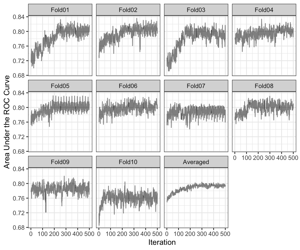
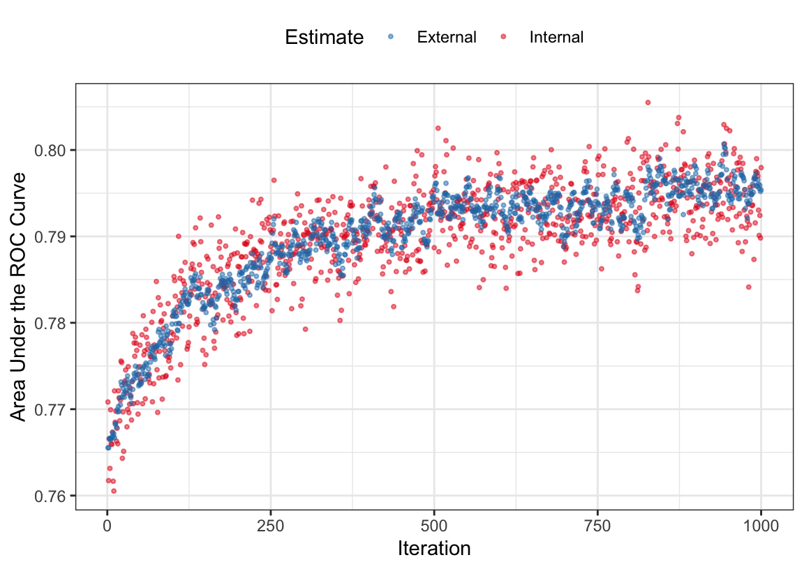
Let’s first look at how the searches did inside each cross-validation iteration. Figure 12.3 shows how the internal ROC estimates changed across the 10 external resamples. The trends vary; some show an increasing trend in performance across iterations while others appear to change very little across iterations. If the initial subset shows good performance, the trend tends to remain flat over iterations. This reflects that there can be substantial variation in the selection process even for data sets with almost 35,000 data points being used within each resample. The last panel shows these values averaged across all resamples.
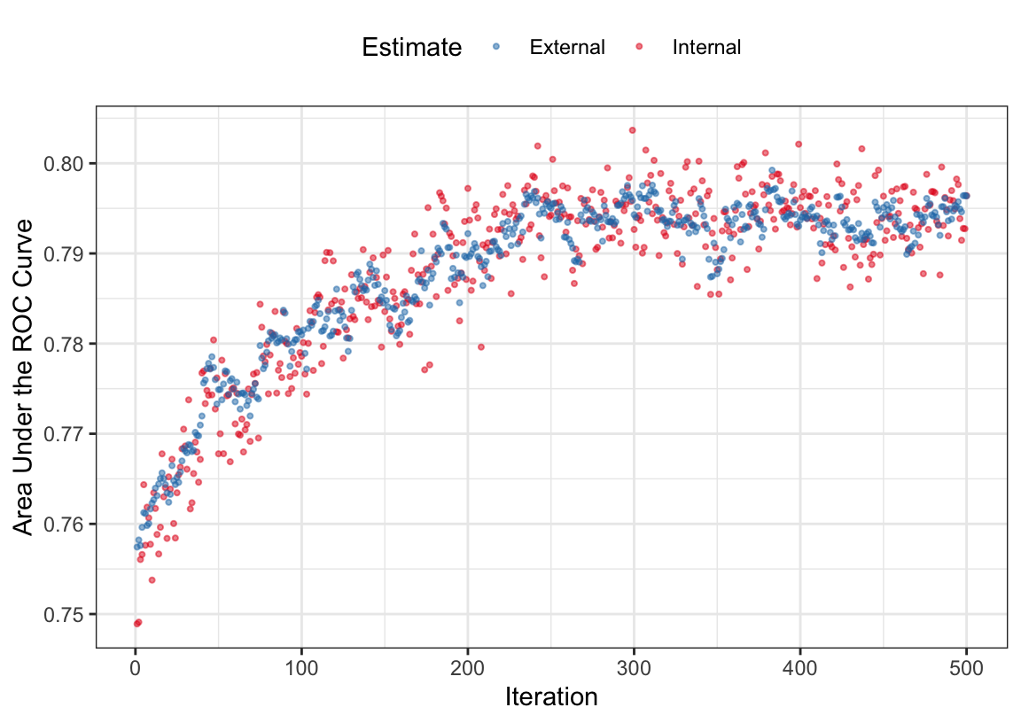
The external resamples also have performance estimates for each iteration. Are these consistent with the inner validation sets? The average rank correlation between the two sets of ROC statistics is 0.6216318 with a range of (0.4299158, 0.8498829). This indicates fairly good consistency. Figure 12.4 overlays the separate internal and external performance metrics averaged across iterations of the search. The cyclical patterns seen in these data reflect the restart feature of the algorithm. The best performance was associated with 383 iterations but it is clear that other choices could be made without damaging performance. Looking at the individual resamples, the optimal iterations ranged from 69 to 404 with an average of 258 iterations. While there is substantial variability in these values, the number of variables selected at those points in the process are more precise; the average was 56 predictors with a range of (49, 64). As will be shown below in Figure 12.7, the size trends across iterations varied with some resamples increasing the number of predictors while others decreased.
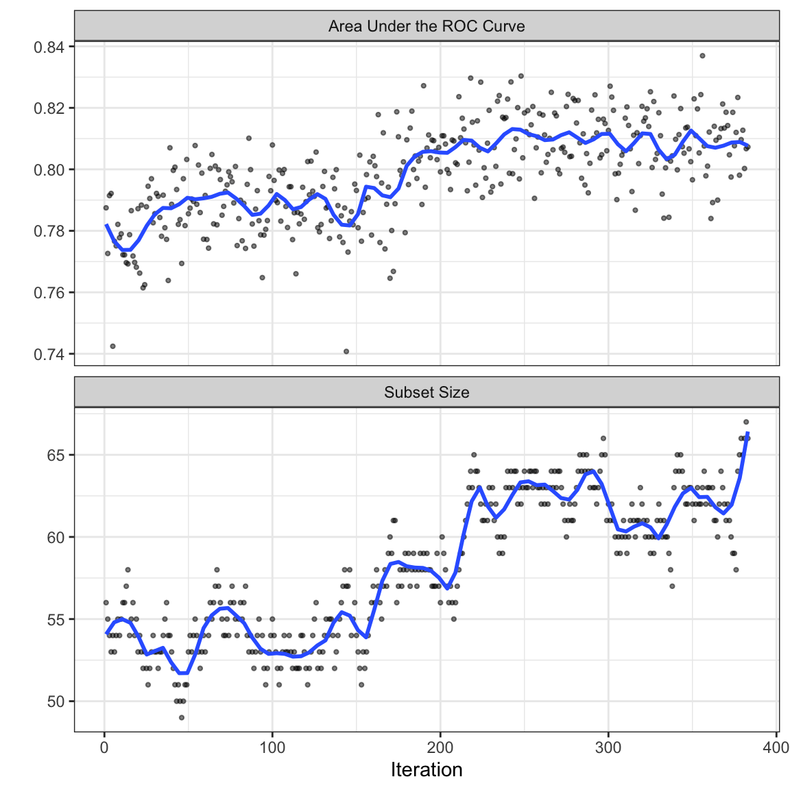
Now that we have a sense of how many iterations of the search are appropriate, let’s look at the final search. For this application of SA, we mimic what was done inside of the external resamples; a validation set of 10% is allocated from the training set and the remainder is used for modeling. Figure 12.5 shows the trends for both the ROC statistic as well as the subset size over the maximum 383 iterations. As the number of iterations increases, subset size trends upwards as does the area under the ROC curve.
In the end, 66 predictors2 (out of a possible 110) were selected and used in the final model:
| diet | education level | height | income | time since last on-line |
| offspring | pets | religion | smokes | town |
| `speaks' C++ fluently | `speaks' C++ okay | `speaks' C++ poorly | lisp | `speaks' lisp poorly |
| black | hispanic/latin | indian | middle eastern | native american |
| other | pacific islander | total essay length | `software` keyword | `engineer` keyword |
| `startup` keyword | `tech` keyword | computers | `engineering` keyword | computer |
| internet | science | technical | web | programmer |
| scientist | code | lol | biotech | matrix |
| geeky | `solving` keyword | teacher | student | silicon |
| law | electronic | mobile | systems | electronics |
| futurama | alot | firefly | valley | lawyer |
| the number of exclamation points | the number of extra spaces | the percentage of lower-case characters | the number of periods | the number of words |
| sentiment score (afinn) | amount of first person words | amount of first person (possessive) words | the number of second-person (possessive) words | the number of `to be' occurances |
| the number of prepositions |
Based on external resampling, our estimate of performance for this model was an ROC AUC of 0.799. This is slightly better than the full model that was estimated in Section 12.1. The main benefit to this process was to reduce the number of predictors. While performance was maintained in this case, performance may be improved in other cases.
A randomization approach was used to investigate if the 52 selected features contained good predictive information. For these data, 100 random subsets of size 66 were generated and used as input to naive Bayes models. The performance of the model from SA was better than 95% of the random subsets. This result indicates that SA selection process approach can be used to find good predictive subsets.
12.2.3 Examining Changes in Performance
Simulated annealing is a controlled random search; the new candidate feature subset is selected completely at random based on the current state. After a sufficient number of iterations, a data set can be created to quantify the difference in performance with and without each predictor. For example, for a SA search lasting 500 iterations, there should be roughly 250 subsets with and without each predictor and each of these has an associated area under the ROC curve computed from the external holdout set. A variety of different analyses can be conducted on these values but the simplest is a basic t-test for equality. Using the SA that was initialized with half of the variables, the 10 predictors with the largest absolute t statistics were (in order): education level, software keyword, engineer keyword, income, the number of words, startup keyword, solving keyword, the number of characters/word, height, and the number of lower space characters. Clearly, a number of these predictors are related and measure characteristics connected to essay length. As an additional benefit to identifying the subset of predictive features, this post hoc analysis can be used to get a clear sense of the importance of the predictors.
12.2.4 Grouped Qualitative Predictors Versus Indicator Variables
Would the results be different if the categorical variables were converted to dummy variables? The same analysis was conducted where the initial models were seeded with half of the predictor set. As with the similar analyses conducted in Section 5.7, all other factors were kept equal. However, since the number of predictors increased from 110 to 298, the number of search iterations was increase from 500 to 1,000 to make sure that all predictors had enough exposure to the selection algorithm. The results are shown in Figure 12.6. The extra iterations were clearly needed to help to achieve a steady state of predictive performance. However, the model performance (AUC: 0.801) was about the same as the approach that kept the categories in a single predictor (AUC: 0.799).
12.2.5 The Effect of the Initial Subset
One additional aspect that is worth considering: how did the subset sizes change within external resamples and would these trends be different if the initial subset had been seeded with more (or fewer) predictors? To answer this, the search was replicated with initial subsets that were either 10% or 90% of the total feature set. Figure 12.7 shows the smoothed subset sizes for each external resample colored by the different initial percentages. In many instances, the two more sparse configurations converged to a subset size that was about half of the total number of possible predictors (although a few showed minimal change overall). A few of the large initial subsets did not substantially decrease. There is some consistency across the three configurations but it does raise the potential issue of how forcefully simulated annealing will try to reduce the number of predictors in the model. Given these results, it may make sense for many practical applications to begin with a small subset size and evaluate performance.
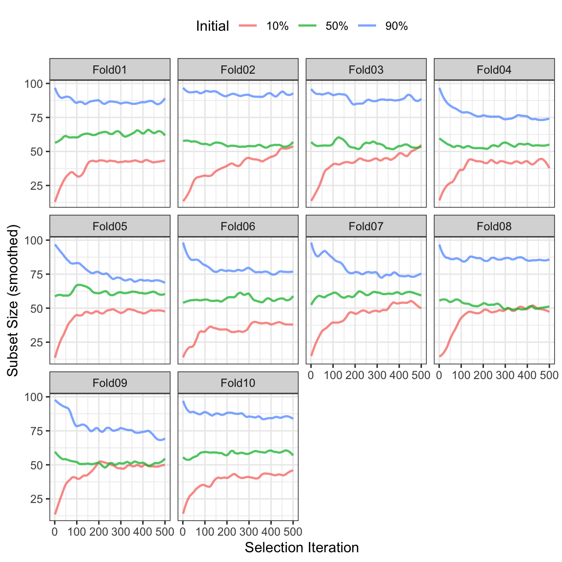
In terms of performance, the areas under the ROC curves for the three sets were 0.805 (10%), 0.799 (50%), and 0.804 (90%). Given the variation in these results, there was no appreciable difference in performance across the different settings.
12.3 Genetic Algorithms
A genetic algorithm (GA) is an optimization tool that is based on concepts of evolution in population biology (Haupt, Haupt, and Haupt 1998; Mitchell 1998). These algorithms have been shown to be able to locate the optimal or near-optimal solutions of complex functions (Mandal, Jeff Wu, and Johnson 2006). To effectively find optimal solutions the algorithm mimics the evolutionary process of a population by generating a candidate set of solutions for the optimization problem, allowing the solutions to reproduce and create new solutions (reproduction), and promoting competition to give the most evolutionarily fit solutions (i.e., optimal) the best chance to survive and populate the subsequent generation (natural selection). This process enables GAs to harness good solutions over time to make better solutions, and has been shown to converge to an optimization plateau (Holland 1992).
The problem of identifying an optimal feature subset is also a complex optimization problem as discussed in Section 10.2. Therefore, if the feature selection problem can be framed in terms of the concepts of evolutionary biology, then the GA engine can be applied to search for optimal feature subsets. In biology, each subject in the population is represented by a chromosome, which is constructed from a sequence of genes. Each chromosome is evaluated based on a fitness criterion. The better the fitnes, the more likely a chromosome will be chosen to use in reproduction to create the next generation of chromosomes. The reproduction stage involves the process of crossover and mutation, where two chromosomes exchange a subset of genes. A small fraction of the offsprings’ genes are then changed due to the process of mutation.
For the purpose of feature selection, the population consists of all possible combinations of features for a particular data set. A chromosome in the population is a specific combination of features (i.e., genes), and the combination is represented by a string which has a length equal to the total number of features. The fitness criterion is the predictive ability of the selected combination of features. Unlike simulated annealing, the GA feature subsets are grouped into generations instead of considering one subset at a time. But a generation in a GAs is similar to an iteration in simulated annealing.
In practice, the initial population of feature subsets needs to be large enough to contain a sufficient amount of diversity across the feature subset space. Often 50 or more randomly selected feature subsets are chosen to seed the initial generation. Our approach is to create random subsets of features that contain between 10% and 90% of the total number of features.
Once the initial generation has been created, the fitness (or predictive ability) of each feature subset is estimated. As a toy example, consider a set of nine predictors (A though I) and an initial population of 12 feature subsets:
| ID | Performance | Probability (%) | |||||||||
|---|---|---|---|---|---|---|---|---|---|---|---|
| 1 | C | F | 0.54 | 6.4 | |||||||
| 2 | A | D | E | F | H | 0.55 | 6.5 | ||||
| 3 | D | 0.51 | 6.0 | ||||||||
| 4 | E | 0.53 | 6.3 | ||||||||
| 5 | D | G | H | I | 0.75 | 8.8 | |||||
| 6 | B | E | G | I | 0.64 | 7.5 | |||||
| 7 | B | C | F | I | 0.65 | 7.7 | |||||
| 8 | A | C | E | G | H | I | 0.95 | 11.2 | |||
| 9 | A | C | D | F | G | H | I | 0.81 | 9.6 | ||
| 10 | C | D | E | I | 0.79 | 9.3 | |||||
| 11 | A | B | D | E | G | H | 0.85 | 10.0 | |||
| 12 | A | B | C | D | E | F | G | I | 0.91 | 10.7 |
Each subset has an associated performance value and, in this case, larger values are better. Next, a subset of these features sets will be selected as parents to reproduce and form the next generation. A logical approach to selecting parents would be to choose the top-ranking features subsets as parents. However, this greedy approach often leads to lingering in a locally optimal solution. To avoid a local optimum, the selection of parents should be a function of the fitness criteria. The most common approach is to select parents is to use a weighted random sample with a probability of selection as a function of predictive performance. A simple way to compute the selection probability is to divide an individual feature subset’s performance value by the sum of all the performance values. The rightmost column in the table above shows the results for this generation.
Suppose subsets 6 and 12 were selected as parents for the next generation. For these parents to reproduce, their genes will undergo a process of crossover and mutation which will result in two new feature subsets. In single-point crossover, a random location between two predictors is chosen3. The parents then exchange features on one side of the crossover point4. Suppose that the crossover point was between predictors D and E represented here:
| ID | |||||||||
|---|---|---|---|---|---|---|---|---|---|
| 6 | B | E | G | I | |||||
| 12 | A | B | C | D | E | F | G | I |
The resulting children of these parents would be:
| ID | |||||||||
|---|---|---|---|---|---|---|---|---|---|
| 13 | B | E | F | G | I | ||||
| 14 | A | B | C | D | E | G | I |
One last modification that can occur for a newly created feature subset is a mutation. A small random probability (1%–2%) is generated for each possible feature. If a feature is selected in the mutation process, then its state is flipped within the current feature subset. This step adds an additional protection to lingering in local optimal solutions. Continuing with the children generated above, suppose that feature I in feature subset 13 was seleted for mutation. Since this feature is already present in subset 13, it would be removed since it was identified for mutation. The resulting children to be evaluated for the next generation would then be:
| ID | |||||||||
|---|---|---|---|---|---|---|---|---|---|
| 13 | B | E | F | G | |||||
| 14 | A | B | C | D | E | G | I |
The process of selecting two parents to generate two more offspring would continue until the new generation is populated.
The reproduction process does not gaurantee that the most fit chromosomes in the current generation will appear in the subsequent generation. This means that there is a chance that the subsequent generation may have less fit chromosomes. To ensure that the subsequent generation maintains the same fitness level, the best chromosome(s) can be carried, as is, into the subsequent generation. This process is called elitism. When elitism is used within a GA, the most fit solution across the observed generations will always be in the final generation. However, this process can cause the GA to linger longer in local optima since the best chromosome will always have the highest probability of reproduction.
12.3.1 External Validation
An external resampling procedure should be used to determine how many iterations of the search are appropriate. This would average the assessment set predictions across all resamples to determine how long the search should proceed when it is directly applied to the entire training set. Basically, the number of iterations is once again a tuning parameter.
A genetic algorithm makes gradual improvements in predictive performance through changes to feature subsets over time. Similar to simulated annealing, an external resampling procedure should be used to select an optimal number of generations. Specifically, GAs are executed within each external resampling loop. Then the internal resamples are used to measure fitness so that different data are used for modeling and evaluation. This process helps prevent the genetic algorithm from finding a feature subset that overfits to the available data, which is a legitimate risk with this type of optimization tool.
Once the number of generations is established, the final selection process is performed on the training set and the best subset is used to filter the predictors for the final model.
To evaluate the performance of GAs for feature selection, we will again use the OkCupid data with a naive Bayes model. In addition, the same data splitting scheme was used as with simulated annealing; 10-fold cross-validation was used for external resampling along with a 10% internal validation set. The search parameters were mostly left to the suggested defaults:
- Generation size: 50,
- Crossover probability: 80%,
- Mutation probability: 1%,
- Elitism: No,
- Number of generations: 145
For this genetic algorithm, it is helpful to examine how the members of each generation (i.e., the feature subsets) change across generations (i.e., search iterations). As we saw before with simulated annealing, simple metrics to understand the algorithm’s characteristics across generations are the feature subset size and the predictive performance estimates. Understanding characteristics of the members within a generation can also be useful. For example, the diversity of the subsets within and between generations can be quantified using a measure such as Jaccard similarity (Tan, Steinbach, and Kumar 2006). This metric is the proportion of the number of predictors in common between two subsets divided by total number of unique predictors in both sets. For example, if there were five possible predictors, the Jaccard similarity between subsets ABC and ABE would be 2/4 or 50%. This value provides insight on how efficiently the generic algorithm is converging towards a common solution or towards potential overfitting.
Figure 12.8 shows curves that monitor the subset size and predictive performance of the current best subset of each generation for each resample. In addition, this figure illustrates the average similarity of the subsets within a generation to the current best subset for each external resample. Several characteristics stand out from this figure. First, despite the resamples having considerable variation in the size of the first generation, they all converge to subset sizes that contain between 61 and 85 predictors. The similarity plot indicates that the subsets within a generation are becoming more similar to the best solution. At the same time, the areas under the ROC curves increase to a value of 0.8427655 at the last generation.
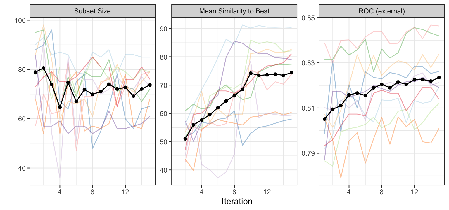
Due to an an overall increasing trend in the average area under the ROC curve, the generation with the largest AUC value was 15. Because the overall trend is still ongoing, additional generations may lead to a more optimal feature subset in a subsequent generation.
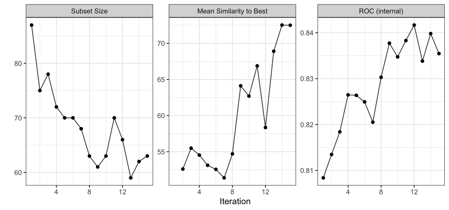
The final search was conducted on the entire training set and Figure 12.9 has the results. These are similar to the internal trends shown previously.
The final predictor set at generation 15 included more variables than the previous SA search and contains the following predictors:
| age | education level | height | income | time since last on-line |
| pets | astrological sign | smokes | town | religion (modifer) |
| astrological sign (modifer) | `speaks' C++ | `speaks' C++ fluently | `speaks' C++ poorly | lisp |
| `speaks' lisp fluently | `speaks' lisp poorly | asian | black | indian |
| middle eastern | native american | other | pacific islander | white |
| total essay length | `software` keyword | `engineer` keyword | `startup` keyword | `tech` keyword |
| computers | `engineering` keyword | computer | internet | technology |
| technical | developer | programmer | scientist | code |
| geek | lol | biotech | matrix | geeky |
| `solving` keyword | problems | data | fixing | teacher |
| student | silicon | law | mechanical | electronic |
| mobile | math | apps | the number of digits | sentiment score (bing) |
| amount of first person words | the number of second-person words | the number of `to be' occurances |
To gauge the effectiveness of the search, 100 random subsets of size 63 were chosen and a naive Bayes model was developed for each. The GA selected subset performed better than 100% of the randomly selected subsets. This indicates that the GA did find a useful subset for predicting the response.
12.3.2 Coercing Sparsity
Genetic algorithms often tend to select larger feature subsets than other methods. This is likely due to the construction of the algorithm in that if a feature is useful for prediction, then it will be included in the feature subset. However, there is less of a penality for keeping a feature that has no impact on predictive performance. This is especially true when coupling a GA with a modeling technique that does not incur a substantial penalty for including irrelevant predictors (Section 10.3). In these cases, adding non-informative predictors does not coerce the selection process to strongly seek sparse solutions.
There are several benefits to a having a sparse solution. First, the model is often simpler, which may make it easier to understand. Fewer predictors also require less computational resources. Is there a way, then, that could be used to compell a search procedure to move towards a more sparse predictor subset solution?
A simple method for reducing the number of predictors is to use a surrogate measure of performance that has an explicit penalty based on the number of features. Section 11.4 introduced the Akaike information criterion (AIC) which augments the objective function with a penalty that is a function of the training set size and the number of model terms. This metric is specifically tailored to models that use the likelihood as the objective (i.e., linear or logistic regression), but cannot be applied to models whose is to optimize other metrics like area under the ROC curve or \(R^2\). Also, AIC usually involves the number of model parameters instead of the number of predictors. For simple parametric regression models, these two quantities are very similar. But there are many models that have no notion of the number of parameters (e.g., trees, \(K\)-NN, etc.), while others can have many more parameters than samples in the training set (e.g., neural networks). However the principle of penalizing the objective based on the number of features can be extended to other models.
Penalizing the measure of performance enables the problem to be framed in terms of multi-parameter optimization (MPO) or multi-objective optimization. There are a variety of appraoches that can be used to solve this issue, including a function to combine many objective values into a final single value. For the purpose of feature selection, one objective is to optimize predictive performance, and the other objective is to include as few features as possible. There are many different options (e.g., Bentley and Wakefield (1998), Xue, Zhang, and Browne (2013), and others) but a simple and straightforward approach is through desirability functions (Harrington 1965; Del Castillo, Montgomery, and McCarville 1996; Mandal et al. 2007). When using this methodology, each objective is translated to a new scale on [0, 1] where larger values are more desirable. For example, an undesirable area under the ROC curve would be 0.50 and a desirable area under the ROC curve would be 1.0. A simple desirability function would be a line that has zero desirability when the AUC is less than or equal to 0.50 and is 1.0 when the AUC is 1.0. Conversely, a desirability function for the number of predictors in the model would be 0.0 when all of the predictors are in the model and would be 1.0 when only one predictor is in the model. Additional desirability functions can be incorporated to guide the modeling process towards other important characteristics.
Once all of the individual desirability functions are defined, the overall desirability statistic is created by taking the geometric mean of all of the individual functions. If there are \(q\) desirability functions \(d_i (i = 1\ldots q)\), the geometric mean is defined as:
\[ D = \left(\prod_{i=1}^q d_j\right)^{1/q} \]
Based on this function, if any one desirability function is unacceptable (i.e., \(d_i = 0\)), the overall measure is also unacceptable6. For feature selection applications, the internal performance metric, which is the one that the genetic algorithm uses to accept or reject subsets, can use the overall desirability to encourage the selection process to favor smaller subsets while still taking performance into account.
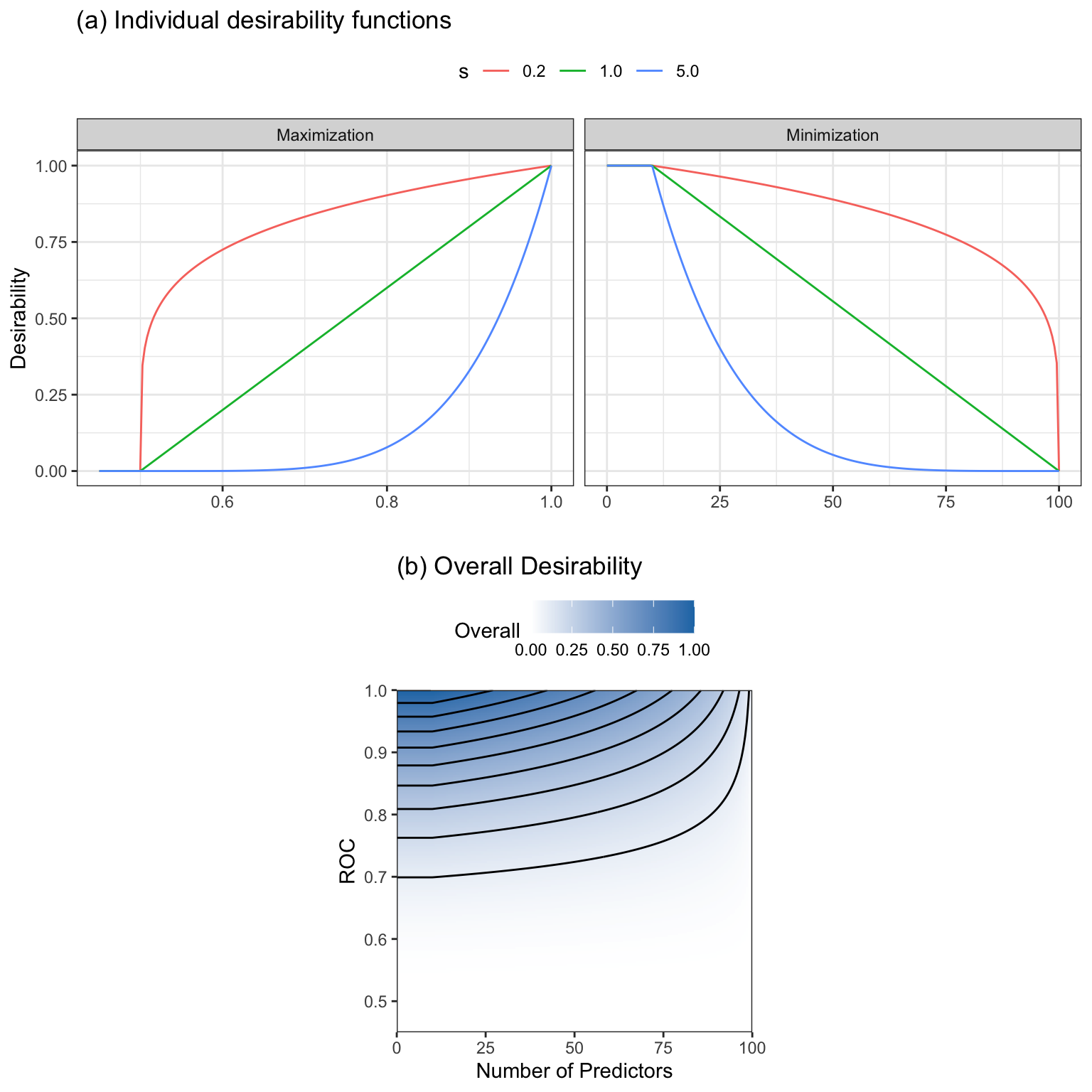
The most commonly used desirability functions for maximizing a quantity use piecewise linear or polynomial functions proposed by Derringer and Suich (1980):
\[\begin{equation} d_i= \begin{cases} 0 &\text{if $x < A$} \\ \left(\frac{x-A}{B-A}\right)^{s} &\text{if $A \leq x \leq B$} \\ 1 &\text{if $x>B$} \end{cases} \end{equation}\]
Figure 12.10(a) shows an example of a maximization function where \(A = 0.50\), \(B = 1.00\), and three different values of the scaling factor \(s\). Note that values of \(s\) less than 1.0 weaken the influence of the desirability function whereas values of \(s > 1.0\) strengthen the influence on the desirability function.
When minimizing a quantity, an analogous function is used:
\[\begin{equation} d_i= \begin{cases} 0 &\text{if $x> B$} \\ \left(\frac{x-B}{A - B}\right)^{s} &\text{if $A \leq x \leq B$} \\ 1 &\text{if $x<A$} \end{cases} \end{equation}\]
Also shown in Figure 12.10(a) is a minimization example of scoring the number of predictors in a subset with values \(A = 10\) and \(B = 100\).
When a maximization function with \(s = 1/5\) and a minimization function with \(s = 1\) are combined using the geometric mean, the results are shown Figure 12.10(b). In this case, the contours are not symmetric since we have given more influence to the area under the ROC curve based on the value of \(s\).
Similar desirability functions exist for cases when a target value is best (i.e., a value between a minimum and maximum), for imposing box constraints, or for using qualitative inputs. Smoother functions could also be used in place of the piecewise equations.
For the OkCupid data, a desirability function with the following objectives was used to guide the GA:
- maximize the area under the ROC curve between \(A = 0.50\) and \(B = 1.00\) with a scale factor of \(s = 2.0\).
- minimize the subset size to be within \(A = 10\) and \(B = 100\) with \(s = 1.0\).
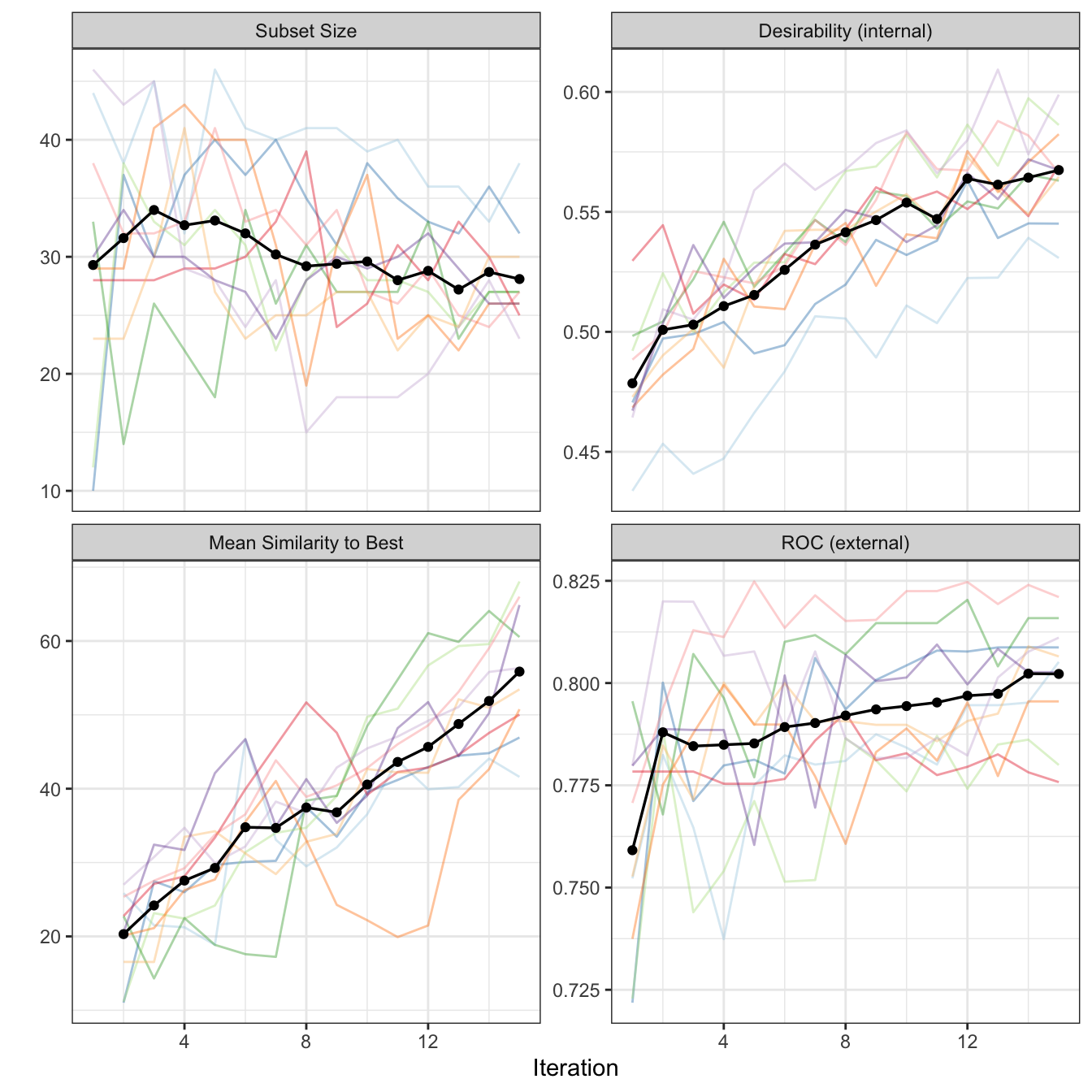
Overall desirability was used for internal performance while the external area under the ROC curve was still used as the primary external metric. Figure 12.11 shows a plot of the internal results similar to Figure 12.8. The overall desirability continually increased and probably would continue to do so with additional generations. The average subset size decreased to be about 28 by the last generation. Based on the averages of the internal resamples, generation 14 was associated with the largest desirability value and with a matching external estimate of the area under the ROC curve of 0.802. This is smaller than the unconstrained GA but the reduced performance is offset by the substantial reduction in the number of of predictors in the model.
For the final run of the genetic algorithm, 32 predictors were chosen at generation 15. These were:
| education level | height | religion | smokes | town |
| `speaks' C++ okay | lisp | `speaks' lisp poorly | asian | native american |
| white | `software` keyword | `engineer` keyword | computers | science |
| programming | technical | code | lol | matrix |
| geeky | fixing | teacher | student | electronic |
| pratchett | math | systems | alot | valley |
| lawyer | the number of punctuation marks |
Depending on the context, a potentially strong argument can be made for a smaller predictor set even if it shows slightly worse results (but better than the full model). If naive Bayes was a better choice than the other models, it would be worth evaluating the normal and sparse GAs on the test set to make a choice.
12.4 Test Set Results
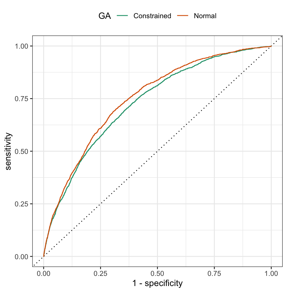
Models were build using the optimal parameter settings for the unconstrained and constrained GAs, and were applied to the test set. The area under the ROC curve for the unconstrained GA was 0.750, while the corresponding value for the constrained GA was 0.731. Both of these values are larger than their analogous resampled estimates, but the two models’ performance rank order in the same way. Figure 12.12 shows that the unconstrained model has uniformly better sensitivity and specificity across the test set cutoffs, although it is difficult to tell if these results are practically different from one another.
12.5 Summary
Global search methods can be an effective tool for investigating the predictor space and identifying subsets of predictors that are optimally related to the response. Despite these methods having some tunable parameters (e.g., the number of iterations, initial subset size, mutation rate, etc.) the default values are sensible and tend to work well.
Although the global search approaches are usually effective at finding good optimal feature sets, they are computationally taxing. For example, the complete process of conducting each of the simulated annealing analyses consisted of fitting a total of 5,501 individual models, and the genetic algorithm analyses required 8,251 models. The independent nature of the folds in external cross-validation allow these methods to be run in parallel, thus reducing the overall computation time. Even so, the GA described above with parallel processing took more than 9 hours when running each external cross-validation fold on a separate core.
In addition, it is important to point out that the naive Bayes model used to compare methods did not require optimization of any tuning parameters7. If the global search methods were used with a radial basis support vector machine (2 tuning parameters) or a C5.0 model (3 tuning parameters), then the computation requirement would rise significantly.
When combining a global search method with a model that has tuning parameters, we recommend that, when possible, the feature set first be winnowed down using expert knowledge about the problem. Next, it is important to identify a reasonable range of tuning parameter values. If a sufficient number of samples are available, a proportion of them can be split off and used to find a range of potentially good parameter values using all of the features. The tuning parameter values may not be the perfect choice for feature subsets, but they should be reasonably effective for finding an optimal subset.
As a general feature selection strategy would be to use models that can intrinsically eliminate features from the model while the model is fit. As previously mentioned, these models may yield good results much more quickly than wrapper methods. The wrapper methods are most useful when a model without this attribute is most appealing. For example, if we had specific reasons to favor naive Bayes models, we would factor the approaches shown in this chapter over more expedient techniques that would automatically filter predictions (e.g., glmnet, MARS, etc.).
12.6 Computing
The website http://bit.ly/fes-global contains R programs for reproducing these analyses.
Chapter References
Bentley, P, and J Wakefield. 1998. “Finding Acceptable Solutions in the Pareto-Optimal Range Using Multiobjective Genetic Algorithms.” In Soft Computing in Engineering Design and Manufacturing, edited by P Chawdhry, R Roy, and R Pant, 231–40. Springer.
Del Castillo, Enrique, Douglas C Montgomery, and Daniel R McCarville. 1996. “Modified Desirability Functions for Multiple Response Optimization.” Journal of Quality Technology 28 (3): 337–45.
Derringer, G, and R Suich. 1980. “Simultaneous optimization of several response variables.” Journal of Quality Technology 12 (4): 214–19.
Harrington, E. 1965. “The Desirability Function.” Industrial Quality Control 21 (10): 494–98.
Haupt, R, S Haupt, and S Haupt. 1998. Practical Genetic Algorithms. Vol. 2. Wiley New York.
Holland, John H. 1992. “Genetic Algorithms.” Scientific American 267 (1): 66–73.
Kirkpatrick, S, D Gelatt, and M Vecchi. 1983. “Optimization by Simulated Annealing.” Science 220 (4598): 671–80.
Mandal, Abhyuday, CF Jeff Wu, and Kjell Johnson. 2006. “SELC: Sequential Elimination of Level Combinations by Means of Modified Genetic Algorithms.” Technometrics 48 (2): 273–83.
Mandal, Abhyuday, Kjell Johnson, CF Jeff Wu, and Dirk Bornemeier. 2007. “Identifying Promising Compounds in Drug Discovery: Genetic Algorithms and Some New Statistical Techniques.” Journal of Chemical Information and Modeling 47 (3): 981–88.
Mitchell, M. 1998. An Introduction to Genetic Algorithms. MIT press.
Spall, J. 2005. Simultaneous Perturbation Stochastic Approximation. John Wiley; Sons.
Tan, PN, M Steinbach, and V Kumar. 2006. Introduction to Data Mining. Pearson Education.
Van Laarhoven, P, and E Aarts. 1987. “Simulated Annealing.” In Simulated Annealing: Theory and Applications, 7–15. Springer.
Wand, M, and C Jones. 1994. Kernel Smoothing. Chapman; Hall/CRC.
Weise, T. 2011. Global Optimization Algorithms - Theory and Application. www.it-weise.de.
Xue, B, M Zhang, and W Browne. 2013. “Particle Swarm Optimization for Feature Selection in Classification: A Multi-Objective Approach.” IEEE Transactions on Cybernetics 43 (6): 1656–71.
Recall that the prior probability was also discussed in Section 3.2.2 when the prevalence was used in some calculations.↩︎
Keyword predictors are shown in .↩︎
There are also multi-point crossover methods that create more than two regions where features are exchanged.↩︎
Often a random probability is also generated to determine if crossover should occur.↩︎
This is a low value for a genetic algorithm. For other applications, the number of generations is usually in the 100’s or 1000’s. However, a value this large would make the feature selection process computationally challenging due to the internal and external validation scheme.↩︎
If we do not want desirability scores to be forced to zero due to just one undesriable characterisitc, then the individual desirability functions can be constrained such that the minimum values are greater than zero.↩︎
The smoothness of the kernel density estimates could have been tuned but this does not typically have a meaningful impact on performance.↩︎