8 Handling Missing Data
Missing data are not rare in real data sets. In fact, the chance that at least one data point is missing increases as the data set size increases. Missing data can occur any number of ways, some of which include the following.
Merging of source data sets: A simple example commonly occurs when two data sets are merged by a sample identifier (ID). If an ID is present in only the first data set, then the merged data will contain missing values for that ID for all of the predictors in the second data set.
Random events: Any measurement process is vulnerable to random events that prevent data collection. Consider the setting where data are collected in a medical diagnostic lab. Accidental misplacement or damage of a biological sample (like blood or serum) would prevent measurements from being made on the sample, thus inducing missing values. Devices that collect actigraphy data can also be affected by random events. For example, if a battery dies or the collection device is damaged then measurements cannot be collected and will be missing in the final data.
Failures of measurement: Measurements based on images require that an image be in focus. Images that are not in focus or are damaged can induce missing values. Another example of a failure of measurement occurs when a patient in a clinical study misses a scheduled physician visit. Measurements that would have been taken for the patient at that visit would then be missing in the final data.
The goal of feature engineering is to get the predictors into a form which models can better utilize in relating the predictors to the response. For example, projection methods (Section 6.3) or autoencoder transformations (Section 6.3.2) for continuous predictors can lead to a significant improvement in predictive performance. Likewise a feature engineering maneuver of likelihood encoding for categorical predictors (Section 5.4) could be predictively beneficial. These feature engineering techniques, as well as many others discussed throughout this work, require that the data have no missing values. Moreover, missing values in the original predictors, regardless of any feature engineering, are intolerable in many kinds of predictive models. Therefore, to utilize predictors or feature engineering techniques, we must first address the missingness in the data. Also, the missingness itself may be an important predictor of the response.
In addition to measurements being missing within the predictors, measurements may also be missing within the response. Most modeling techniques cannot utilize samples that have missing response values in the training data. However a new approach known as semi-supervised learning has the ability to utilize samples with unknown response values in the training set. Semi-supervised learning methods are beyond the scope of this chapter; for further reference see Zhu and Goldberg (2009). Instead this chapter will focus on methods for resolving missing values within the predictors.
Types of Missing Data
The first and most important question when encountering missing data is “why are these values missing?” Sometimes the answer might already be known or could be easily inferred from studying the data. If the data stem from a scientific experiment or clinical study, information from laboratory notebooks or clinical study logs may provide a direct connection to the samples collected or to the patients studied that will reveal why measurements are missing. But for many other data sets, the cause of missing data may not be able to be determined. In cases like this, we need a framework for understanding missing data. This framework will, in turn, lead to appropriate techniques for handling the missing information.
One framework to view missing values is through the lens of the mechanisms of missing data. Three common mechanisms are:
Structural deficiencies in the data
Random occurrences, or
Specific causes.
A structural deficiency can be defined as a missing component of a predictor that was omitted from the data. This type of missingness is often the easiest to resolve once the necessary component is identified. The Ames housing data provides an example of this type of missingness in the Alley predictor. This predictor takes values of “gravel” or “paved”, or is missing. Here, 93.2 percent of homes have a missing value for alley. It may be tempting to simply remove this predictor because most of the values are missing. However doing this would throw away valuable predictive information of home price since missing, in this case, means that the property has no alley. A better recording for the Alley predictor might be to replace the missing values with “No Alley Access”.
A second reason for missing values is due to random occurrences. Little and Rubin (2014) subdivide this type of randomness into two categories:
Missing completely at random (MCAR): the likelihood of a missing results is equal for all data points (observed or unobserved). In other words, the missing values are independent of the data. This is the best case situation.
Missing at random (MAR): the likelihood of a missing results is not equal for all data points (observed or unobserved). In this scenario, the probability of a missing result depends on the observed data but not on the unobserved data.
In practice it can be very difficult or impossible to distinguish if the missing values have the same likelihood of occurrence for all data, or have different likelihoods for observed or unobserved data. For the purposes of this text, the methods described herein can apply to either case. We refer the reader to Little and Rubin (2014) for a deeper understanding of these nuanced cases.
A third mechanism of missing data is missingness due to a specific cause (or not missing at random (NMAR) (Little and Rubin 2014)). This type of missingness often occurs in clinical studies where patients are measured periodically over time. For example, a patient may drop out of a study due to an adverse side effect of a treatment or due to death. For this patient, no measurements will be recorded after the time of drop-out. Data that are not missing at random are the most challenging to handle. The techniques presented here may or may not be appropriate for this type of missingness. Therefore, we must make a good effort to understanding the nature of the missing data prior to implementing any of the techniques described below.
This chapter will illustrate ways for assessing the nature and severity of missing values in the data, highlight models that can be used when missing values are present, and review techniques for removing or imputing missing data.
For illustrations, we will use the Chicago train ridership data (Chapter 4) and the scat data from Reid (2015) (previously seen in Section 6.3.3). The latter data set contains information on animal droppings that were collected in the wild. A variety of measurements were made on each sample including morphological observations (i.e., shape), location/time information, and laboratory tests. The DNA in each sample was genotyped to determine the species of the sample (gray fox, coyote, or bobcat). The goal for these data is to build a predictive relationship between the scat measurements and the species. After gathering a new scat sample, the model would be used to predict the species that produced the sample. Out of the 110 collected scat samples, 19 had one or more missing predictor values.
8.1 Understanding the Nature and Severity of Missing Information
As illustrated throughout this book, visualizing data are an important tool for guiding us towards implementing appropriate feature engineering techniques. The same principle holds for understanding the nature and severity of missing information throughout the data. Visualizations as well as numeric summaries are the first step in grasping the challenge of missing information in a data set. For small to moderate data (100’s of samples and 100’s of predictors), several techniques are available that allow the visualization of all of the samples and predictors simultaneously for understanding the degree and location of missing predictor values. When the number of samples or predictors become large, the missing information must first be appropriately condensed and then visualized. In addition to visual summaries, numeric summaries are a valuable tool for diagnosing the nature and degree of missingness.
Visualizing Missing Information
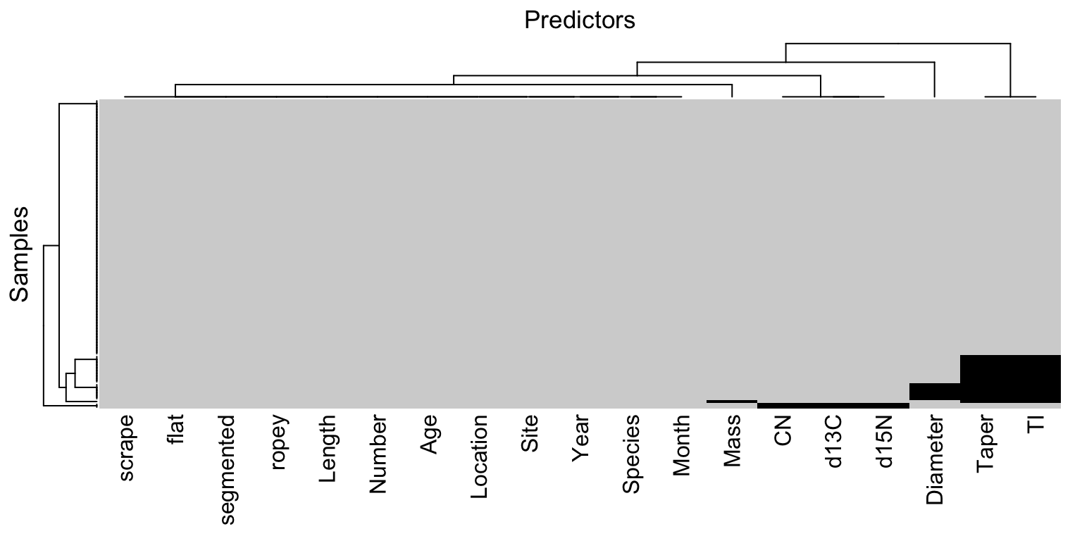
When the training set has a moderate number of samples and predictors, a simple method to visualize the missing information is with a heatmap. In this visualization the figure has two colors representing the present and missing values. The top of Figure 8.1 illustrates a heatmap of missing information for the animal scat data. The heatmap visualization can be reorganized to highlight commonalities across missing predictors and samples using hierarchical cluster analysis on the predictors and on the samples (Dillon and Goldstein 1984). This visualization illustrates that most predictors and samples have complete or nearly complete information. The three morphological predictors (diameter, taper, and taper index) are more frequently missing. Also two samples are missing all three of the laboratory measurements (d13N, d15N, and CN).
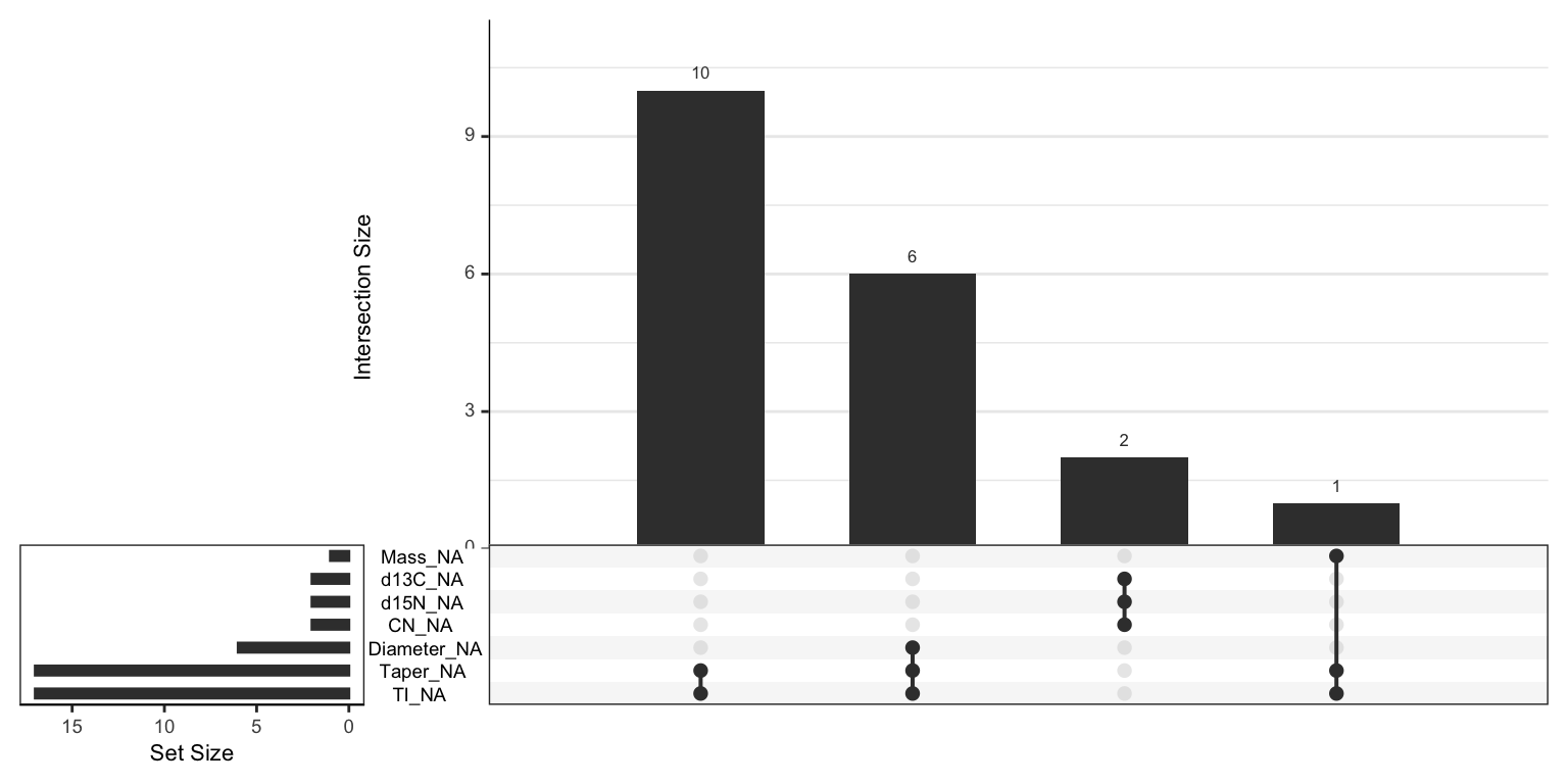
A co-occurrence plot can further deepen the understanding of missing information. This type of plot displays the frequency of missing predictor combinations (Figure 8.1). As the name suggests, a co-occurrence plot displays the frequencies of the most common missing predictor combinations. The figure makes it easy to see that TI, Tapper, and Diameter have the most missing values, that Tapper and TI are missing together most frequently, and that six samples are missing all three of the morphological predictors. The bottom of Figure 8.1 displays the co-occurrence plot for the scat data.
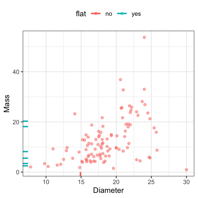
In addition to exploring the global nature of missing information, it is wise to explore relationships within the data that might be related to missingness. When exploring pairwise relationships between predictors, missing values of one predictor can be called out on the margin of the alternate axis. For example, Figure 8.2 shows the relationship between the diameter and mass of the feces. Hash marks on either axis represent samples that have an observed value for that predictor but have a missing value for the corresponding predictor. The points are colored by whether the sample was a “flat puddle that lacks other morphological traits.” Since the missing diameter measurements have this unpalatable quality, it makes sense that some shape attributes cannot be determined. This can be considered to be structurally missing, but there still may be a random or informative component to the missingness.
However, in relation to the outcome, the six flat samples were spread across the gray fox (\(n=5\)) and coyote (\(n=1\)) data. Given the small sample size, it is unclear if this missingness is related to the outcome (which would be problematic). Subject-matter experts would need to be consulted to understand if this is the case.
When the data has a large number of samples or predictors, using heatmaps or co-occurrence plots are much less effective for understanding missingness patterns and characteristics. In this setting, the missing information must first be condensed prior to visualization. Principal component analysis (PCA) was first illustrated in Section 6.3 as a dimension reduction technique. It turns out that PCA can also be used to visualize and understand the samples and predictors that have problematic levels of missing information. To use PCA in this setting, the predictor matrix is converted to a binary matrix where a zero represents a non-missing value and a one represents a missing value. Because PCA searches for directions that summarize maximal variability, the initial dimensions capture variation caused by the presence of missing values. Samples that do not have any missing values will be projected onto the same location close to the origin. Alternatively, samples with missing values will be projected away from the origin. Therefore by simply plotting the scores of the first two dimensions, we can begin to identify the nature and degree of missingness in large data sets.
The same approach can be applied to understanding the degree of missingness among the predictors. To do this, the binary matrix representing missing values is first transposed so that predictors are now in the rows and the samples are in the columns. PCA is then applied to this matrix and the resulting dimensions now capture variation cause by the presence of missing values across the predictors.
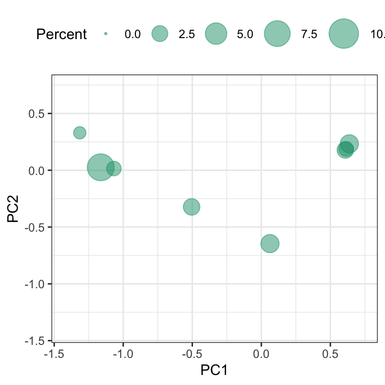
To illustrate this approach, we will return to the Chicago train ridership data which has ridership values for 5,733 days and 146 stations. The missing data matrix can be represented by dates and stations. Applying PCA to this matrix generates the first two components illustrated in Figure 8.3. Points in the plot are sized by the amount of missing stations. In this case each day had at least one station that had a missing value, and there were 8 distinct missing data patterns.
Further exploration found that many of the missing values occurred during September 2013. The cause of these missing values should be investigated further.
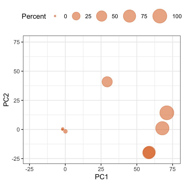
To further understand the degree and location of missing values, the data matrix can be transformed and PCA applied again. Figure 8.4 presents the scores for the stations. Here points are labeled by the amount of missing information across stations. In this case, 5 stations have a substantial amount of missing data. The root cause of missing values for these stations should be investigated to better determine an appropriate way for handing these stations.
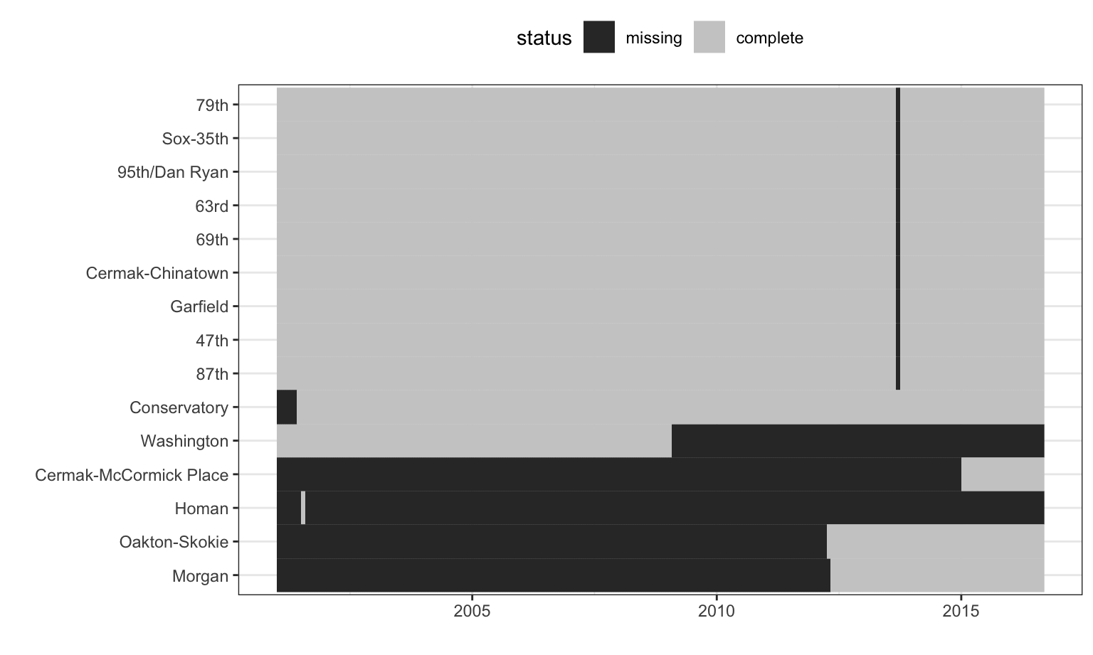
The stations with excessive missingness and their missing data patterns over time are shown in Figure 8.5. The station order is set using a clustering algorithm while the x-axis is ordered by date. There are nine stations whose data are almost complete except for a single month gap. These stations are all on the Red Line and occur during the time of the Red Line Reconstruction Project that affected stations north of Cermak-Chinatown to the 95th Street station. The Homan station only has one month of complete data and was replaced by the Conservatory station which opened in 2001, which explains why the Conservatory station has missing data prior to 2001. Another anomaly appears for the Washington-State station. Here the data collection ceased midway through the data set because the station was closed in the mid-2000s. The further investigation of the missing data indicates that these patterns are unrelated to ridership and are mostly due structural causes.
Summarizing Missing Information
Simple numerical summaries are effective at identifying problematic predictors and samples when the data become too large to visually inspect. On a first pass, the total number or percent of missing values for both predictors and samples can be easily computed. Returning to the animal scat data, Table 8.1 presents the predictors by amount of missing values. Similarly, Table 8.2 contains the samples by amount of missing values. These summaries can then be used for investigating the underlying reasons why values are missing or as a screening mechanism for removing predictors or samples with egregious amounts of missing values.
| Percent Missing (%) | Predictor |
|---|---|
| 0.9090909 | Mass |
| 1.8181818 | d13C, d15N, and CN |
| 5.4545455 | Diameter |
| 15.4545455 | Taper and TI |
| Percent Missing (%) | Sample |
|---|---|
| 10.52632 | 51, 68, 69, 70, 71, 72, 73, 75, 76, and 86 |
| 15.78947 | 11, 13, 14, 15, 29, 60, 67, 80, and 95 |
8.2 Models that are Resistant to Missing Values
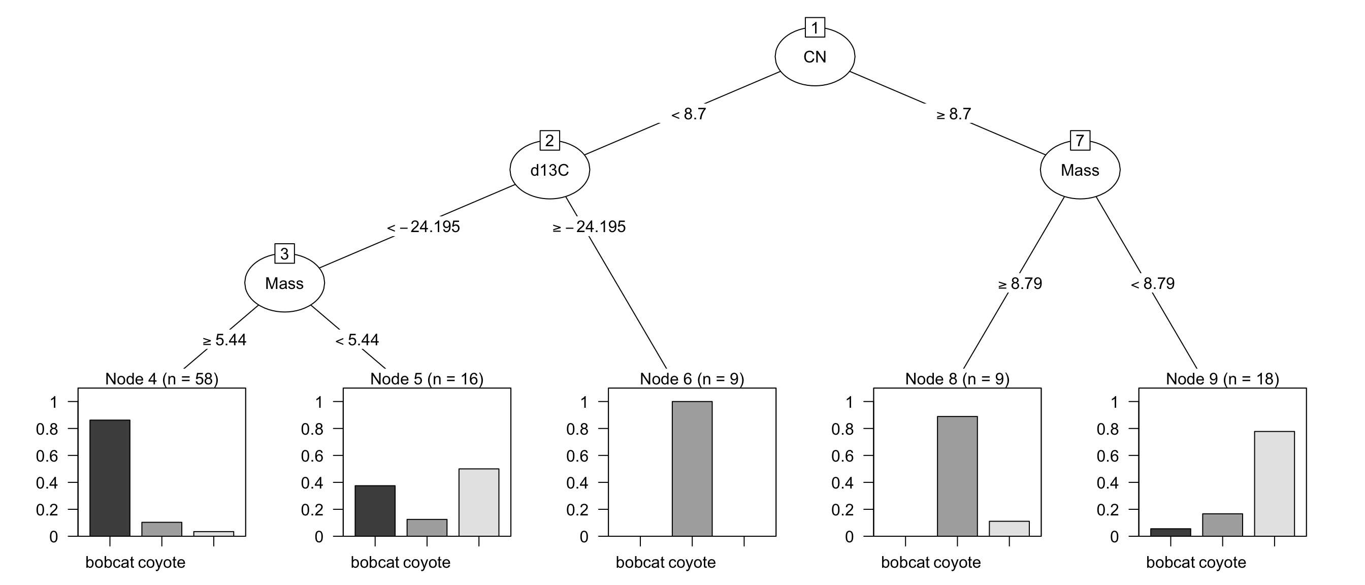
Many popular predictive models such as support vector machines, the glmnet, and neural networks, cannot tolerate any amount of missing values. However, there are a few predictive models that can internally handle incomplete data1. Certain implementations of tree-based models have clever procedures to accommodate incomplete data. The CART methodology (Breiman et al. 1984) uses the idea of surrogate splits. When creating a tree, a separate set of splits are cataloged (using alternate predictors than the current predictor being split) that can approximate the original split logic if that predictor value is missing. Figure 8.6 displays the recursive partitioning model for the animal scat data. All three predictors selected by the tree contain missing values as illustrated in Figure 8.1. The initial split is based on the carbon/nitrogen ratio (CN < 8.7). When a sample has a missing value for CN, then the CART model uses an alternative split based on the indicator for whether the scat was flat or not. These two splits result in the same partitions for 80.6% of the data of the data and could be used if the carbon/nitrogen ratio is missing. Moving further down the tree, the surrogate predictors for d13C and Mass are Mass and d13C, respectively. This is possible since these predictors are not simultaneously missing.
C5.0 (Quinlan 1993; Kuhn and Johnson 2013) takes a different approach. Based on the distribution of the predictor with missing data, fractional counts are used in subsequent splits. For example, this model’s first split for the scat data is d13C > 24.55. When this statement is true, all 13 training set samples are coyotes. However, there is a single missing value for this predictor. The counts of each species in subsequent nodes are then fractional due to adjusting for the number of missing values for the split variable. This allows the model to keep a running account of where the missing values might have landed in the partitioning.
Another method that can tolerate missing data is Naive Bayes. This method models the class-specific distributions of each predictor separately. Again, if the missing data mechanism is not pathological, then these distribution summaries can use the complete observations for each individual predictor and will avoid case-wise deletion.
8.3 Deletion of Data
When it is desirable to use models that are intolerant to missing data, then the missing values must be extricated from the data. The simplest approach for dealing with missing values is to remove entire predictor(s) and/or sample(s) that contain missing values. However, one must carefully consider a number of aspects of the data prior to taking this approach. For example, missing values could be eliminated by removing all predictors that contain at least one missing value. Similarly, missing values could be eliminated by removing all samples with any missing values. Neither of these approaches will be appropriate for all data as can be inferred from the “No Free Lunch” theorem. For some data sets, it may be true that particular predictors are much more problematic than others; by removing these predictors, the missing data issue is resolved. For other data sets, it may be true that specific samples have consistently missing values across the predictors; by removing these samples, the missing data issue is likewise resolved. In practice, however, specific predictors and specific samples contain a majority of the missing information.
Another important consideration is the intrinsic value of samples as compared to predictors. When it is difficult to obtain samples or when the data contain a small number of samples (i.e., rows), then it is not desirable to remove samples from the data. In general, samples are more critical than predictors and a higher priority should be placed on keeping as many as possible. Given that a higher priority is usually placed on samples, an initial strategy would be to first identify and remove predictors that have a sufficiently high amount of missing data. Of course, predictor(s) in question that are known to be valuable and/or predictive of the outcome should not be removed. Once the problematic predictors are removed, then attention can focus on samples that surpass a threshold of missingness.
Consider the Chicago train ridership data as an example. The investigation into these data earlier in the chapter revealed that several of the stations had a vast amount of contiguous missing data (Figure 8.5). Every date (sample) had at least one missing station (predictor), but the degree of missingness across predictors was minimal. However, a handful of stations had excessive missingness. For these stations there is too much contiguous missing data to keep the stations in the analysis set. In this case it would make more sense to remove the handful of stations. It is less clear for the stations on the Red Line as to whether or not to keep these in the analysis sets. Given the high degree of correlation between stations, it was decided that excluding all stations with missing data from all of the analyses in this text would not be detrimental to building an effective model for predicting ridership at the Clark-Lake station. This example illustrates that there are several important aspects to consider when determining the approach for handling missing values.
Besides throwing away data, the main concern with removing samples (rows) of the training set is that it might bias the model that relates the predictors to the outcome. A classic example stems from medical studies. In these studies, a subset of patients are randomly assigned to the current standard of care treatment while another subset of patients are assigned to a new treatment. The new treatment may induce an adverse effect for some patients, causing them to drop out of the study thus inducing missing data for future clinical visits. This kind of missing data is clearly not missing at random and the elimination of these data from an analysis would falsely measure the outcome to be better than it would have if their unfavorable results had been included. That said, Allison (2001) notes that if the data are missing completely at random, this may be a viable approach.
8.4 Encoding Missingness
When a predictor is discrete in nature, missingness can be directly encoded into the predictor as if it were a naturally occurring category. This makes sense for structurally missing values such as the example of alleys in the Ames housing data. Here, it is sensible to change the missing values to a category of “no alley.” In other cases, the missing values could simply be encoded as “missing” or “unknown.” For example, Kuhn and Johnson (2013) use a data set where the goal is to predict the acceptance or rejection of grant proposals. One of the categorical predictors was grant sponsor which took values such as “Australian competitive grants”, “cooperative research centre”, “industry”, etc.. In total, there were more than 245 possible values for this predictor with roughly 10% of the grant applications having an empty sponsor value. To enable the applications that had an empty sponsor to be used in modeling, empty sponsor values were encoded as “unknown”. For many of the models that were investigated, the indicator for an unknown sponsor was one of the most important predictors of grant success. In fact, the odds-ratio that contrasted known versus unknown sponsor was greater than 6. This means that it was much more likely for a grant to be successfully funded if the sponsor predictor was unknown. In fact, in the training set the grant success rate associated with an unknown sponsor was 82.2% versus 42.1% for a known sponsor.
Was encoding the missing values a successful strategy? Clearly, the mechanism that led to the missing sponsor label being identified as strongly associated with grant acceptance was genuinely important. Unfortunately, it is impossible to know why this association is so important. The fact that something was going on here is important and this encoding helped identify its occurrence. However, it would be troublesome to accept this analysis as final and imply some sort of cause-and-effect relationship2. A guiding principle that can be used to determine if encoding missingness is a good idea is to think about how the results would be interpreted if that piece of information becomes important to the model.
8.5 Imputation Methods
Another approach to handling missing values is to impute or estimate them. Missing value imputation has a long history in statistics and has been thoroughly researched. Good places to start are Little and Rubin (2014), Van Buuren (2012) and Allison (2001). In essence, imputation uses information and relationships among the non-missing predictors to provide an estimate to fill in the missing value.
Historically, statistical methods for missing data have been concerned with the impact on inferential models. In this situation, the characteristics and quality of the imputation strategy have focused on the test statistics that are produced by the model. The goal of these techniques is to ensure that the statistical distributions are tractable and of good enough quality to support subsequent hypothesis testing. The primary approach in this scenario is to use multiple imputations; several variations of the data set are created with different estimates of the missing values. The variations of the data sets are then used as inputs to models and the test statistic replicates are computed for each imputed data set. From these replicate statistics, appropriate hypothesis tests can be constructed and used for decision making.
There are several differences between inferential and predictive models that impact this process:
- In many predictive models, there is no notion of distributional assumptions (or they are often intractable). For example, when constructing most tree-based models, the algorithm does not require any specification of a probability distribution to the predictors. As such, many predictive models are incapable of producing inferential results even if that were a primary goal3. Given this, traditional multiple imputation methods may not have relevance for these models.
- Many predictive models are computationally expensive. Repeated imputation would greatly exacerbate computation time and overhead. However, there is an interest in capturing the benefit (or detriment) caused by an imputation procedure. To ensure that the variation imparted by the imputation is captured in the training process, we recommend that imputation be performed within the resampling process.
- Since predictive models are judged on their ability to accurately predict yet-to-be-seen samples (including the test set and new unknown samples), as opposed to statistical appropriateness, it is critical that the imputed values be as close as possible to their true (unobserved) values.
- The general focus of inferential models is to thoroughly understand the relationships between the predictor and response for the available data. Conversely, the focus of predictive models is to understand the relationships between the predictors and the response that are generalizable to yet-to-be-seen samples. Multiple imputation methods do not keep the imputation generator after the missing data have been estimated which provides a challenge for applying these techniques to new samples.
The last point underscores the main objective of imputation with machine learning models: produce the most accurate prediction of the missing data point. Some other important characteristics that a predictive imputation method should have are:
Within a sample data point, other variables may also be missing. For this reason, an imputation method should be tolerant of other missing data.
Imputation creates a model embedded within another model. There is a prediction equation associated with every predictor in the training set that might have missing data. It is desirable for the imputation method to be fast and have a compact prediction equation.
Many data sets often contain both numeric and qualitative predictors. Rather than generating dummy variables for qualitative predictors, a useful imputation method would be able to use predictors of various types as inputs.
The model for predicting missing values should be relatively (numerically) stable and not be overly influenced by outlying data points.
Virtually any predictive model could be used to impute the data. Here, the focus will be on several that are good candidates to consider.
Imputation does beg the question of how much missing data are too much to impute? Although not a general rule in any sense, 20% missing data within a column might be a good “line of dignity” to observe. Of course, this depends on the situation and the patterns of missing values in the training set.
It is also important to consider that imputation is probably the first step in any preprocessing sequence. Imputing qualitative predictors prior to creating indicator variables so that the binary nature of the resulting imputations can be preserved is a good idea. Also, imputation should usually occur prior to other steps that involve parameter estimation. For example, if centering and scaling is performed on data prior to imputation, the resulting means and standard deviations will inherit the potential biases and issues incurred from data deletion.
K-Nearest Neighbors
When the training set is small or moderate in size, \(K\)-nearest neighbors can be a quick and effective method for imputing missing values (Eskelson et al. 2009; Tutz and Ramzan 2015). This procedure identifies a sample with one or more missing values. Then it identifies the \(K\) most similar samples in the training data that are complete (i.e., have no missing values in some columns). Similarity of samples for this method is defined by a distance metric. When all of the predictors are numeric, standard Euclidean distance is commonly used as the similarity metric. After computing the distances, the \(K\) closest samples to the sample with the missing value are identified and the average value of the predictor of interest is calculated. This value is then used to replace the missing value of the sample.
Often, however, data sets contain both numeric and categorical predictors. If this is the case, then Euclidean distance is not an appropriate metric. Instead, Gower’s distance is a good alternative (Gower 1971). This metric uses a separate specialized distance metric for both the qualitative and quantitative predictors. For a qualitative predictor, the distance between two samples is 1 if the samples have the same value and 0 otherwise. For a quantitative predictor \(x\), the distance between samples \(i\) and \(j\) is defined as
\[d(x_i, x_j) = 1- \frac{|x_i-x_j|}{R_x}\]
where \(R_x\) is the range of the predictor. The distance measure is computed for each predictor and the average distance is used as the overall distance. Once the \(K\) neighbors are found, their values are used to impute the missing data. The mode is used to impute qualitative predictors and the average or median is used to impute quantitative predictors. \(K\) can be a tunable parameter, but values around 5–10 are a sensible default.
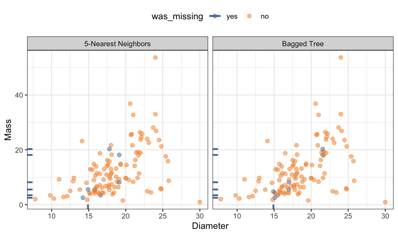
For the animal scat data, Figure 8.7 shows the same data from Figure 8.2 but with the missing values filled in using 5 neighbors based on Gower’s distance. The new values mostly fall around the periphery of these two dimensions but are within the range of the samples with complete data.
Trees
Tree-based models are a reasonable choice for an imputation technique since a tree can be constructed in the presence of other missing data4. In addition, trees generally have good accuracy and will not extrapolate values beyond the bounds of the training data. While a single tree could be used as an imputation technique, it is known to produce results that have low bias but high variance. Ensembles of trees, however, provide a low-variance alternative. Random forests is one such technique and has been studied for this purpose (Stekhoven and Buhlmann 2011). However, there are a couple of notable drawbacks when using this technique in a predictive modeling setting. First and foremost, the random selection of predictors at each split necessitates a large number of trees (500 to 2000) to achieve a stable, reliable model. Each of these trees is unpruned and the resulting model usually has a large computational footprint. This can present a challenge as the number of predictors with missing data increases since a separate model must be built and retained for each predictor. A good alternative that has a smaller computational footprint is a bagged tree. A bagged tree is constructed in a similar fashion to a random forest. The primary difference is that in a bagged model, all predictors are evaluated at each split in each tree. The performance of a bagged tree using 25–50 trees is generally in the ballpark of the performance of a random forest model. And the smaller number of trees is a clear advantage when the goal is to find reasonable imputed values for missing data.
Figure 8.7 illustrates the imputed values for the scat data using a bagged ensemble of 50 trees. When imputing the diameter predictor was the goal, the estimated RMSE of the model was 4.16 (or an \(R^2\) of 13.6%). Similarly, when imputing the mass predictor was the goal, the estimated RMSE was 8.56 (or an \(R^2\) of 28.5%). The RMSE and \(R^2\) metrics are not terribly impressive. However, these imputations from the bagged models produce results that are reasonable, are within the range of the training data, and allow the predictors to be retained for modeling (as opposed to case-wise deletion).
Linear Methods
When a complete predictor shows a strong linear relationship with a predictor that requires imputation, a straightforward linear model may be the best approach. Linear models can be computed very quickly and have very little retained overhead. While a linear model does require complete predictors for the imputation model, this is not a fatal flaw since the model coefficients (i.e., slopes) use all of the data for estimation. Linear regression can be used for a numeric predictor that requires imputation. Similarly, logistic regression is appropriate for a categorical predictor that requires imputation.
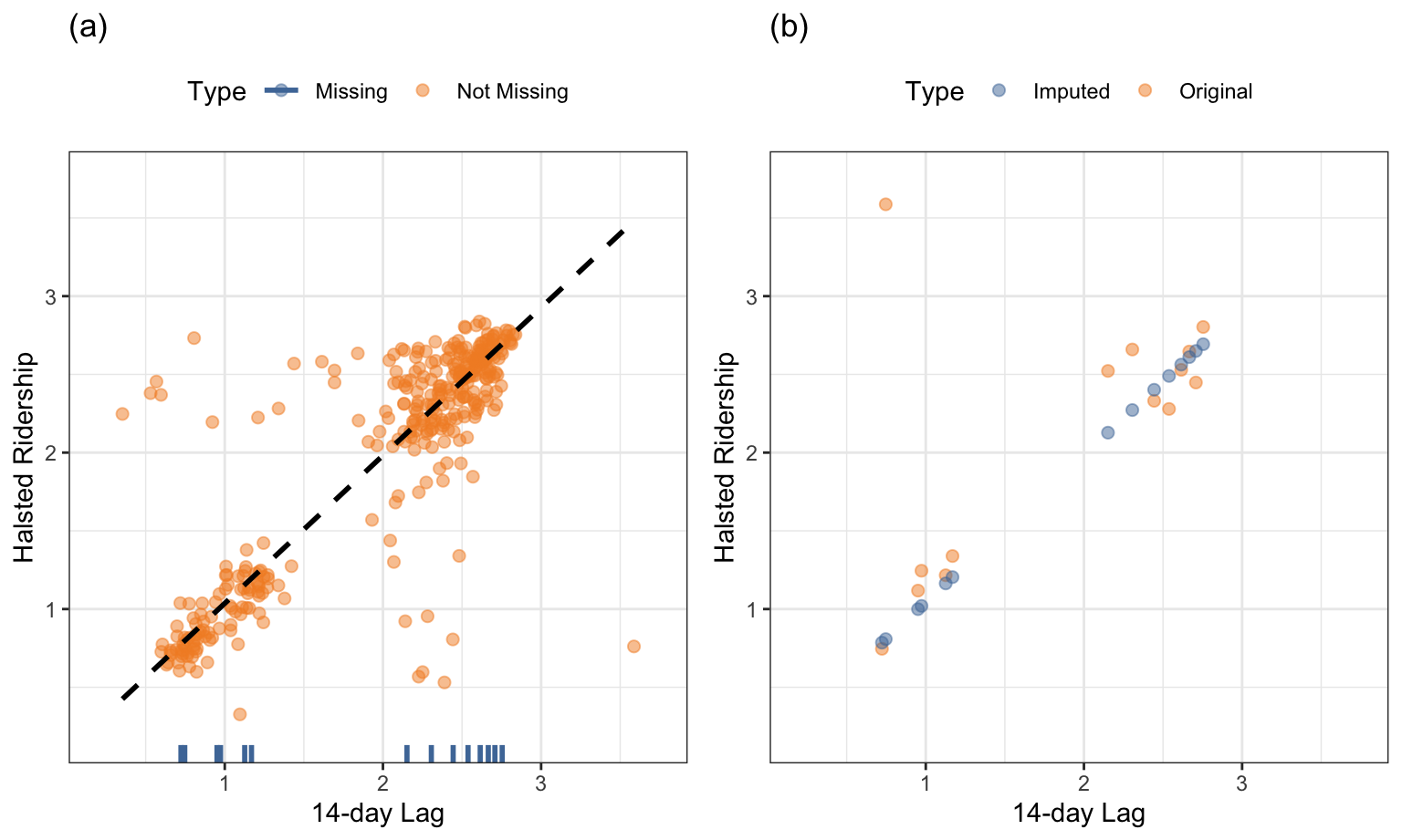
The Chicago train ridership data will be used to illustrate the usefulness of a simple technique like linear regression for imputation. It is conceivable that one or more future ridership values might be missing in random ways from the complete data set. To simulate potential missing data, missing values have been induced for ridership at the Halsted stop. As illustrated previously in Figure 4.7, the 14-day lag in ridership within a stop is highly correlated with the current day’s ridership. Figure 8.8(a) displays the relationship between these predictors for the Halsted stop in 2010 with the missing values of the current day highlighted on the x-axis. The majority of the data displays a linear relationship between these predictors, with a handful of days having values that are away from the overall trend. The fit of a robust linear model to these data is represented by the dashed line. Figure 8.8(b) compares the imputed values with the original true ridership values. The robust linear model performs adequately at imputing the missing values, with the exception of one day. This day had unusual ridership because it was a holiday. Including holiday as a predictor in the robust model would help improve the imputation.
The concept of linear imputation can be extended to high-dimensional data. Audigier, Husson, and Josse (2016), for example, have developed methodology to impute missing data based on similarity measures and principal components analysis.
8.6 Special Cases
There are situations where a data point isn’t missing but is also not complete. For example, when measuring the duration of time until an event, it might be known that the duration is at least some time \(T\) (since the event has not occurred). These types of values are referred to as censored5. A variety of statistical methods have been developed to analyze this type of data.
Durations are often right censored since the terminating value is not known. In other cases, left censoring can occur. For example, laboratory measurements may have a lower limit of detection, which means that the measuring instrument cannot reliably quantify values below a threshold \(X\). This threshold is usually determined experimentally in the course of developing the measurement system. When a predictor has values below the lower limit of detection, the these values are usually reported as “\(<X\)”. When these data are to be included in a predictive model, there is usually a question of how to handle the censored values. A widely accepted practice is to use the lower limit value of \(X\) as the result. While this would not adversely affect some partitioning models, such as trees or rules, it may have a detrimental impact on other models since it assumes that these are the true values. Censored values affect metrics that measure the variability. Specifically, the variability will be underestimated. This effect is similar in a manner to binning in Section 6.2.2, and the model may overfit to a cluster of data points with the same value.
To mitigate the variability issue, left censored values can be imputed using random uniform values between zero and \(X\). In cases where there is good information about the distribution below \(X\), other random value assignment schemes can be used that better represent the distribution. For example, there may be some scientific or physiological reason that the smallest possible value is greater than zero (but less than \(X\)). While imputing in this fashion adds random noise to the data, it is likely to be preferable to the potential overfitting issues that can occur by assigning a value of \(X\) to the data.
Another atypical situation occurs when the data have a strong time component. In this case, to preserve these characteristics of the data, simple moving average smoothers can be used to impute the data so that any temporal effects are not disrupted. As previously mentioned in Section 6.1, care most be taken on the ends so that the test (or other) data are not used to impute the training set values.
8.7 Summary
Missing values are common occurrences in data. Unfortunately, most predictive modeling techniques cannot handle any missing values. Therefore, this problem must be addressed prior to modeling. Missing data may occur due to random chance or due to a systematic cause. Understanding the nature of the missing values can help to guide the decision process about how best to remove or impute the data.
One of the best ways to understand the amount and nature of missing values is through an appropriate visualization. For smaller data sets, a heatmap or co-occurrence plot is helpful. Larger data sets can be visualized by plotting the first two scores from a PCA model of the missing data indicator matrix.
Once the severity of missing values is known, then a decision needs to be made about how to address these values. When there is a severe amount of missing data within a predictor or a sample, it may be prudent to remove the problematic predictors or samples. Alternatively, if the predictors are qualitative, missing values could be encoded with a category of “missing”.
For small to moderate amounts of missingness, the values can be imputed. There are many types of imputation techniques. A few that are particularly useful when the ultimate goal is to build a predictive model are k-nearest neighbors, bagged trees, and linear models. Each of these methods have a relatively small computation footprint and can be computed quickly which enables them to be included in the resampling process of predictive modeling.
8.8 Computing
The website http://bit.ly/fes-missing contains R programs for reproducing these analyses.
Chapter References
Allison, P. 2001. Missing Data. Sage Publications.
Audigier, Vincent, François Husson, and Julie Josse. 2016. “A Principal Component Method to Impute Missing Values for Mixed Data.” Advances in Data Analysis and Classification 10 (1): 5–26.
Breiman, L., J. Friedman, R. Olshen, and C. Stone. 1984. Classification and Regression Trees. New York: Chapman; Hall.
Dillon, W, and M Goldstein. 1984. Multivariate Analysis Methods and Applications. Wiley.
Eskelson, B, H Temesgen, V Lemay, TT Barrett, N Crookston, and A Hudak. 2009. “The Roles of Nearest Neighbor Methods in Imputing Missing Data in Forest Inventory and Monitoring Databases.” Scandinavian Journal of Forest Research 24 (3): 235–46.
Gower, J. 1971. “A General Coefficient of Similarity and Some of Its Properties.” Biometrics, 857–71.
Kuhn, M, and K Johnson. 2013. Applied Predictive Modeling. Springer.
Little, R, and D Rubin. 2014. Statistical Analysis with Missing Data. John Wiley; Sons.
Quinlan, R. 1993. C4.5: Programs for Machine Learning. Morgan Kaufmann Publishers.
Reid, R. 2015. “A Morphometric Modeling Approach to Distinguishing Among Bobcat, Coyote and Gray Fox Scats.” Wildlife Biology 21 (5): 254–62.
Stekhoven, D, and P Buhlmann. 2011. “MissForest - Non-Parametric Missing Value Imputation for Mixed-Type Data.” Bioinformatics 28 (1): 112–18.
Tutz, G, and S Ramzan. 2015. “Improved Methods for the Imputation of Missing Data by Nearest Neighbor Methods.” Computational Statistics and Data Analysis 90: 84–99.
Van Buuren, S. 2012. Flexible Imputation of Missing Data. Chapman; Hall/CRC.
Zhu, Xiaojin, and Andrew B Goldberg. 2009. “Introduction to Semi-Supervised Learning.” Synthesis Lectures on Artificial Intelligence and Machine Learning 3 (1): 1–130.
This is true provided that the mechanism that causes the missing data are not pathological.↩︎
A perhaps more difficult situation would be explaining to the consumers of the model that “We know that this is important but we don’t know why!”↩︎
Obviously, there are exceptions such as linear and logistic regression, Naive Bayes models, etc.↩︎
However, many implementations do not have this property.↩︎
In cases where the data are not defined outside of lower or upper bounds, the data would be considered truncated.↩︎