4 Exploratory Visualizations
The driving goal in everything that we do in the modeling process is to find reproducible ways to explain the variation in the response. As discussed in the previous chapter, discovering patterns among the predictors that are related to the response involves selecting a resampling scheme to protect against overfitting, choosing a performance metric, tuning and training multiple models, and comparing model performance to identify which models have the best performance. When presented with a new data set, it is tempting to jump directly into the predictive modeling process to see if we can quickly develop a model that meets the performance expectations. Or, in the case where there are many predictors, the initial goal may be to use the modeling results to identify the most important predictors related to the response. But as illustrated in Figure 1.4, a sufficient amount of time should be spent exploring the data. The focus of this chapter will be to present approaches for visually exploring data and to demonstrate how this approach can be used to help guide feature engineering.
One of the first steps of the exploratory data process when the ultimate purpose is to predict a response is to create visualizations that help elucidate knowledge of the response and then to uncover relationships between the predictors and the response. Therefore our visualizations should start with the response, understanding the characteristics of its distribution, and then to build outward from that with the additional information provided in the predictors. Knowledge about the response can be gained by creating a histogram or box plot. This simple visualization will reveal the amount of variation in the response and if the response was generated by a process that has unusual characteristics that must be investigated further. Next, we can move on to exploring relationships among the predictors and between predictors and the response. Important characteristics can be identified by examining
- scatter plots of individual predictors and the response,
- a pairwise correlation plot among the predictors,
- a projection of high-dimensional predictors into a lower dimensional space,
- line plots for time-based predictors,
- the first few levels of a regression or classification tree,
- a heatmap across the samples and predictors, or
- mosaic plots for examining associations among categorical variables.
These visualizations provide insights that should be used to inform the initial models. It is important to note that some of the most useful visualizations for exploring the data are not necessarily complex or difficult to create. In fact, a simple scatter plot can elicit insights that a model may not be able to uncover, and can lead to the creation of a new predictor or to a transformation of a predictor or the response that improves model performance. The challenge here lies in developing intuition for knowing how to visually explore data to extract information for improvement. As illustrated in Figure 1.4, exploratory data analysis should not stop at this point, but should continue after initial models have been built. Post model building, visual tools can be used to assess model lack-of-fit and to evaluate the potential effectiveness of new predictors that were not in the original model.
In this chapter, we will delve into a variety of useful visualization tools for exploring data prior to constructing the initial model. Some of these tools can then be used after the model is built to identify features that can improve model performance. Following the outline of Figure 1.4, we will look at visualizations prior to modeling, then during the modeling process. We also refer the reader to Tufte (1990), Cleveland (1993), and Healy (2018) which are excellent resources for visualizing data.
To illustrate these tools, the Chicago Train Ridership data will be used for numeric visualizations and the OkCupid data for categorical visualizations.
4.1 Introduction to the Chicago Train Ridership Data
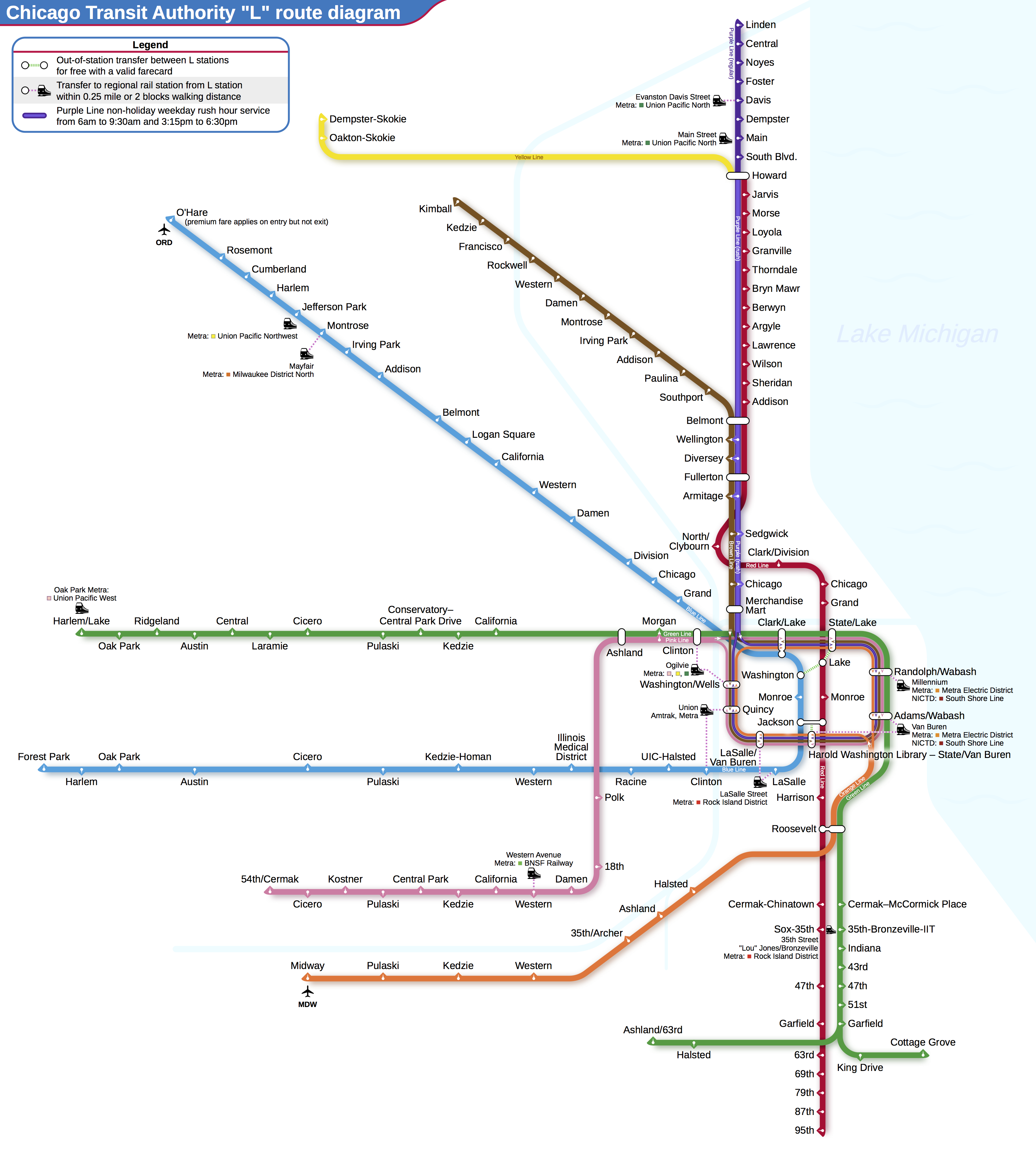
To illustrate how exploratory visualizations are a critical part of understanding a data set and how visualizations can be used to identify and uncover representations of the predictors that aid in improving the predictive ability of a model, we will be using data collected on ridership on the Chicago Transit Authority (CTA) “L” train system1 (Figure 4.1). In the short term, understanding ridership over the next one or two weeks would allow the CTA to ensure that an optimal number of cars were available to service the Chicagoland population. As a simple example of demand fluctuation, we would expect that ridership in a metropolitan area would be stronger on weekdays and weaker on weekends. Two common mistakes of misunderstanding demand could be made. At one extreme, having too few cars on a line to meet weekday demand would delay riders from reaching their destination and would lead to overcrowding and tension. At the other extreme, having too many cars on the weekend would be inefficient leading to higher operational costs and lower profitability. Good forecasts of demand would help the CTA to get closer to optimally meeting demand.
In the long term, forecasting could be used to project when line service may be necessary, to change the frequency of stops to optimally service ridership, or to add or eliminate stops as populations shift and demand strengthens or weakens.
For illustrating the importance of exploratory visualizations, we will focus on short-term forecasting of daily ridership. Daily ridership data were obtained for 126 stations2 between January 22, 2001 and September 11, 2016. Ridership is measured by the number of entries into a station across all turnstiles, and the number of daily riders across stations during this time period varied considerably, ranging between 0 and 36,323 per day. For ease of presentation, ridership will be shown and analyzed in units of thousands of riders.
Our illustration will narrow to predicting daily ridership at the Clark/Lake stop. This station is an important stop to understand; it is located in the downtown loop, has one of the highest riderships across the train system, and services four different lines covering northern, western, and southern Chicago.
For these data, the ridership numbers for the other stations might be important to the models. However, since the goal is to predict future ridership volume, only historical data would be available at the time of prediction. For time series data, predictors are often formed by lagging the data. For this application, when predicting day \(D\), predictors were created using the lag–14 data from every station (e.g., ridership at day \(D-14\)). Other lags can also be added to the model, if necessary.
Other potential regional factors that may affect public transportation ridership are the weather, gasoline prices, and the employment rate. For example, it would be reasonable to expect that more people would use public transportation as the cost of using personal transportation (i.e., gas prices) increase for extended periods of time. Likewise, the use of public transportation would likely increase as the unemployment rate decreases. Weather data were obtained for the same time period as the ridership data. The weather information was recorded hourly and included many conditions such as overcast, freezing rain, snow, etc.. A set of predictors were created that reflects conditions related to rain, snow/ice, clouds, storms, and clear skies. Each of these categories is determined by pooling more granular recorded conditions. For example, the rain predictor reflects recorded conditions that included “rain,” “drizzle,” and “mist”. New predictors were encoded by summarizing the hourly data across a day by calculating the percentage of observations within a day where the conditions were observed. As an illustration, on December 20, 2012, conditions were recorded as snowy (12.8% of the day), cloudy (15.4%), as well as stormy (12.8%), and rainy (71.8%). Clearly, there is some overlap in the conditions that make up these categories, such as cloudy and stormy.
Other hourly weather data were also available related to the temperature, dew point, humidity, air pressure, precipitation and wind speeds. Temperature was summarized by the daily minimum, median, and maximum as well as the daily change. Pressure change was similarly calculated. In most other cases, the median daily value was used to summarize the hourly records. As with the ridership data, future weather data are not available so lagged versions of these data were used in the models3. In total, there were 18 weather-related predictors available. Summarization of these types of data are discussed more in Chapter 9.
In addition to daily weather data, average weekly gasoline prices were obtained for the Chicago region (U.S. Energy Information Administration 2017a) from 2001 through 2016. For the same time period, monthly unemployment rates were pulled from United States Census Bureau (2017). The potential usefulness of these predictors will be discussed below.
4.2 Visualizations for Numeric Data: Exploring Train Ridership Data
4.2.1 Box Plots, Violin Plots, and Histograms
Univariate visualizations are used to understand the distribution of a single variable. A few common univariate visualizations are box-and-whisker plots (i.e., box plot), violin plots, or histograms. While these are simple graphical tools, they provide great value in comprehending characteristics of the quantity of interest.
Because the foremost goal of modeling is to understand variation in the response, the first step should be to understand the distribution of the response. For a continuous response such as the ridership at the Clark/Lake station, it is important to understand if the response has a symmetric distribution, if the distribution has a decreasing frequency of larger observations (i.e., the distribution is skewed), if the distribution appears to be made up of two or more individual distributions (i.e., the distribution has multiple peaks or modes), or if there appears to be unusually low or high observations (i.e outliers).
Understanding the distribution of the response as well as its variation provides a lower bound of the expectations of model performance. That is, if a model contains meaningful predictors, then the residuals from a model that contains these predictors should have less variation than the variation of the response. Furthermore, the distribution of the response may indicate that the response should be transformed prior to analysis. For example, responses that have a distribution where the frequency of response proportionally decreases with larger values may indicate that the response follows a log-normal distribution. In this case, log-transforming the response would induce a normal (bell-shaped, symmetric) distribution and often will enable a model to have better predictive performance. A third reason why we should work to understand the response is because the distribution may provide clues for including or creating features that help explain the response.
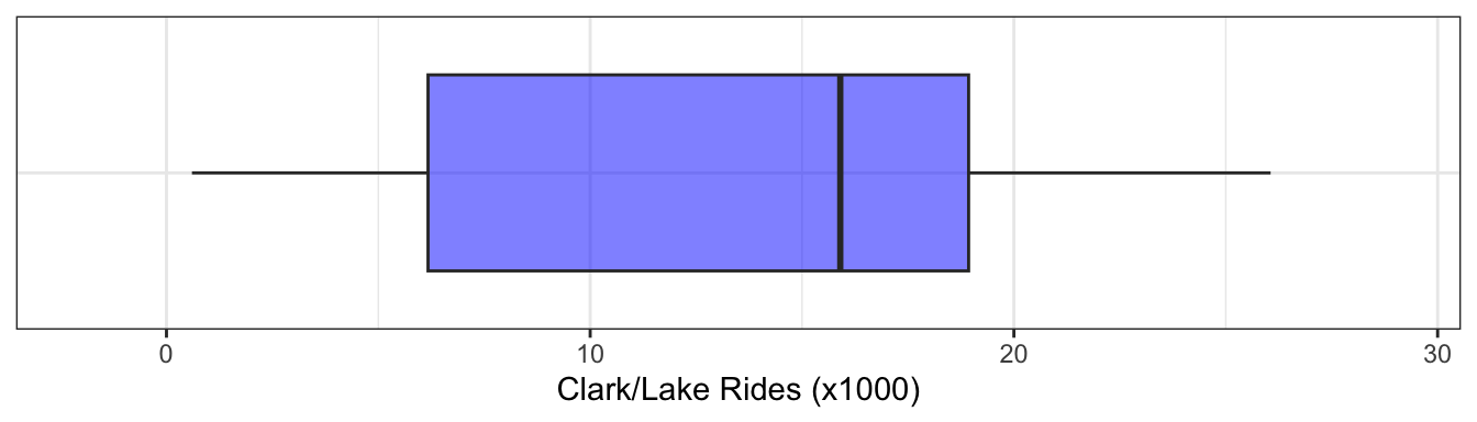
As a simple example of the importance of understanding the response distribution, consider Figure 4.2 which displays a box plot of the response for the ridership at the Clark/Lake station. The box plot was originally developed by John Tukey as a quick way to assess a variable’s distribution (Tukey 1977), and consists of the minimum, lower quartile, median, upper quartile and maximum of the data. Alternative versions of the box plot extend the whiskers to a value beyond which samples would be considered unusually high (or low) (Frigge, Hoaglin, and Iglewicz 1989). A variable that has a symmetric distribution has equal spacing across the quartiles making the box and whiskers also appear symmetric. Alternatively, a variable that has fewer values in a wider range of space will not appear symmetric.
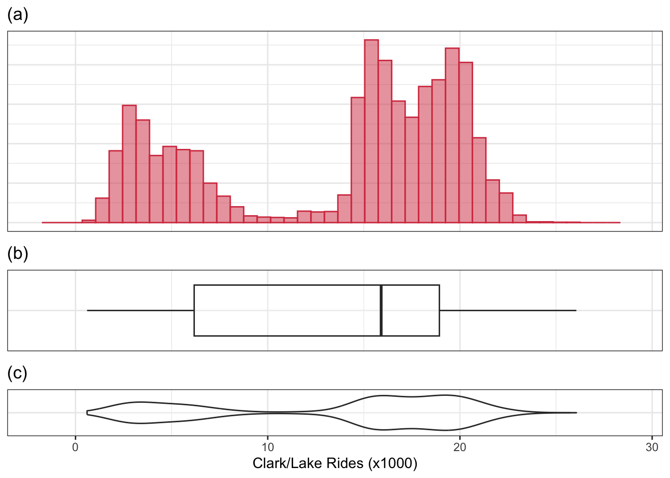
A drawback of the box plot is that it is not effective at identifying distributions that have multiple peaks or modes. As an example, consider the distribution of ridership at the Clark/Lake station (Figure 4.3). Part (a) of this figure is a histogram of the data. To create a histogram, the data are binned into equal regions of the variable’s value. The number of samples are counted in each region, and a bar is created with the height of the frequency (or percentage) of samples in that region. Like box plots, histograms are simple to create, and these figures offer the ability to see additional distributional characteristics. In the ridership distribution, there are two peaks, which could represent two different mechanisms that affect ridership. The box plot (b) is unable to capture this important nuance. To achieve a compact visualization of the distribution that retains histogram-like characteristics, Hintze and Nelson (1998) developed the violin plot. This plot is created by generating a density or distribution of the data and its mirror image. Figure 4.3 (c) is the violin plot, where we can now see the two distinct peaks in ridership distribution. The lower quartile, median, and upper quartile can be added to a violin plot to also consider this information in the overall assessment of the distribution.
These data will be analyzed in several chapters. Given the range of the daily ridership numbers, there was some question as to whether the outcome should be modeled in the natural units or on the log scale. On one hand, the natural units makes interpretation of the results easier since the RMSE would be in terms of riders. However, if the outcome were transformed prior to modeling, it would ensure that negative ridership could not be predicted. The bimodal nature of these data, as well as distributions of ridership for each year that have a longer tail on the right made this decision difficult. In the end, a handful of models were fit both ways to make the determination. The models computed in the natural units appeared to have slightly better performance and, for this reason, all models were analyzed in the natural units.
Examining the distribution of each predictor can help to guide our decisions about the need to engineer the features through transformation prior to analysis. When we have a moderate number of predictors (< ~100) and when the predictors are on the same order of magnitude, we can visualize the distributions simultaneously using side-by-side box or violin plots. Consider again the ridership data with the two-week lag in ridership as predictors. The distributions across selected stations for weekday ridership for 2016 are provided in ?fig-eda-rides-distribution. Here, our focus is on the variability and range of ridership across stations. Despite the earlier warning, box plots are good at characterizing these aspects of data. To help see patterns more clearly, ridership is ordered from the largest median (left) to the smallest median (right). Several characteristics stand out: variability in ridership increases with the median ridership, there are a number of unusually low and unusually high values for each station, and a few stations have distinctly large variation. One station particularly stands out, which is about one-quarter of the way from the left. This happens to be the Addison station which is the nearest stop to Wrigley Field. The wider distribution is due to ridership associated with the weekday home games for the Chicago Cubs, with attendance at its peak reaching close to the most frequently traveled stations. If the goal was to predict ridership at the Addison station, then the Cubs’ home game schedule would be important information for any model. The unusually low values for the majority of the stations will be discussed next.
As the number of predictors grows, the ability to visualize the individual distributions lessens and may be practically impossible. In this situation, a subset of predictors that are thought to be important can be examined using these techniques.
4.2.2 Augmenting Visualizations Through Faceting, Colors, and Shapes
Additional dimensions can be added to almost any figure by using faceting, colors, and shapes. Faceting refers to creating the same type of plot (e.g., a scatter plot) and splitting the plot into different panels based on some variable4. Figure 3.2 is a good example. While this is a simple approach, these types of augmentation can be powerful tools for seeing important patterns that can be used to direct the engineering of new features. The Clark/Lake station ridership distribution is a prime candidate for adding another dimension. As shown above, Figure 4.3 has two distinct peaks. A reasonable explanation for this would be that ridership is different for weekdays than for weekends. Figure 4.4 partitions the ridership distribution by part of the week through color and faceting (for ease of visualization). Part of the week was not a predictor in the original data set; by using intuition and carefully examining the distribution, we have found a feature that is important and necessary for explaining ridership and should be included in a model.
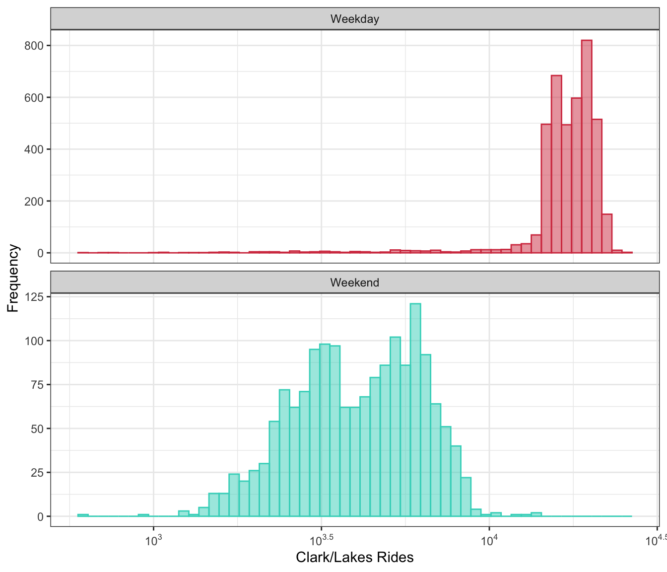
Figure 4.4 invites us to pursue understanding of these data further. Careful viewing of the weekday ridership distribution should draw our eye to a long tail on the left which is a result of a number of days with lower ridership similar to the range of ridership on weekends. What would cause weekday ridership to be low? If the cause can be uncovered, then a feature can be engineered. A model that has the ability to explain these lower values will have better predictive performance than a model that does not.
The use of colors and shapes for elucidating predictive information will be illustrated several of the following sections.
4.2.3 Scatter Plots
Augmenting visualizations through the use of faceting, color, or shapes is one way to incorporate an additional dimension in a figure. Another approach is to directly add another dimension to a graph. When working with two numeric variables, this type of graph is called a scatter plot. A scatter plot arranges one variable on the x-axis and another on the y-axis. Each sample is then plotted in this coordinate space. We can use this type of figure to assess the relationship between a predictor and the response, to uncover relationships between pairs of predictors, and to understand if a new predictor may be useful to include in a model. These simple relationships are the first to provide clues to assist in engineering characteristics that may not be directly available in the data.
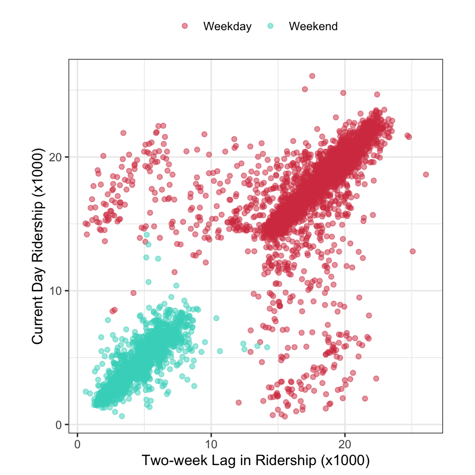
If the goal is to predict ridership at the Clark/Lake station then we could anticipate that recent past ridership information should be related to current ridership. That is to say another potential predictor to consider would be the previous day’s or previous week’s ridership information. Because we know that weekday and weekend have different distributions, a one-day lag would be less useful for predicting ridership on Monday or Saturday. A week-based lag would not have this difficulty (although it would be further apart in time) since the information occurs on the same day of the week. Because the primary interest is in predicting ridership two weeks in advance, we will create the 14-day lag in ridership for the Clark/Lake station.
In this case, the relationship between these variables can be directly understood by creating a scatter plot (Figure 4.5). This figure highlights several characteristics that we need to know: there is a strong linear relationship between the 14-day lag and current-day ridership, there are two distinct groups of points (due to the part of the week), and there are many 14-day lag/current day pairs of days that lie far off from the overall scatter of points. These results indicate that the 14-day lag will be a crucial predictor for explaining current-day ridership. Moreover, uncovering the explanation of samples that are far off from the overall pattern visualized here will lead to a new feature that will be useful as a input to models.
4.2.4 Heatmaps
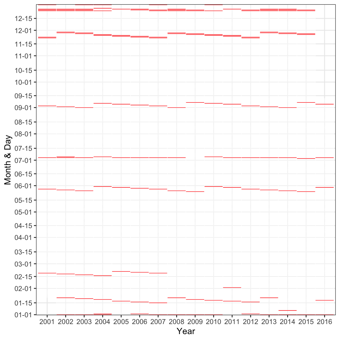
Low weekday ridership as illustrated in Figure 4.4 might be due to annual occurrences; to investigate this hypothesis, the data will need to be augmented. The first step is to create an indicator variable for weekdays with ridership less than 10,000 or greater than or equal to 10,000. We then need a visualization that allows us to see when these unusual values occur. A visualization that would elucidate annual patterns in this context is a heatmap. A heatmap is a versatile plot that can be created utilizing almost any type of predictor and displays one predictor on the x-axis and another predictor on the y-axis. In this figure the x- and y-axis predictors must be able to be categorized. The categorized predictors then form a grid, and the grid is filled by another variable. The filling variable can be either continuous or categorical. If continuous, then the boxes in the grid are colored on a continuous scale from the lowest value of the filling predictor to the highest value. If the filling variable is categorical, then the boxes have distinct colors for each category.
For the ridership data, we will create a month and day predictor, a year predictor, and an indicator of weekday ridership less than 10,000 rides.
These new features are the inputs to the heatmap (Figure 4.6). In this figure, the x-axis represents the year and the y-axis represents the month and day. Red boxes indicate weekdays that have ridership less than 10,000 for the Clark/Lake station. The heatmap of the data in this form brings out some clear trends. Low ridership occurs on or around the beginning of the year, mid-January, mid-February until 2007, late-May, early-July, early-September, late-November, and late-December. Readers in the US would recognize these patterns as regularly observed holidays. Because holidays are known in advance, adding a feature for common weekday holidays will be beneficial for models to explain ridership.
Carefully observing the heatmap points to two days that do not follow the annual patterns: February 2, 2011 and January 6, 2014. These anomalies were due to extreme weather. On February 2, 2011, Chicago set a record low temperature of -16F. Then on January 6, 2014, there was a blizzard that dumped 21.2 inches of snow on the region. Extreme weather instances are infrequent, so adding this predictor will have limited usefulness in a model. If the frequency of extreme weather increases in the future, then using forecast data could become a valuable predictor for explaining ridership.
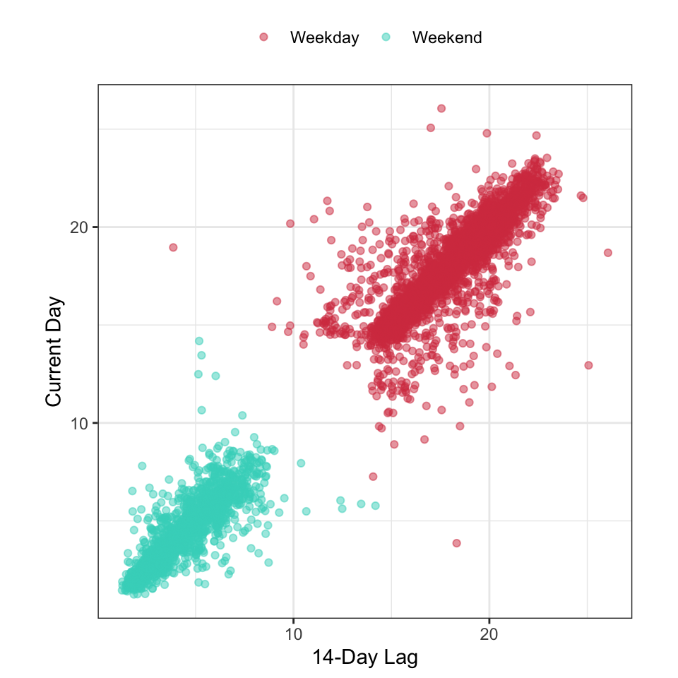
Now that we understand the effect of major US holidays, these values will be excluded from the scatter plot of 14-day lag versus current-day ridership (Figure 4.7). Most of the points that fell off the diagonal of Figure 4.5 are now gone. However a couple of points remain. The day associated with these points was June 11, 2010 which was the city’s celebration for the Chicago Blackhawks winning the Stanley Cup. While these types of celebrations are infrequent, engineering a feature to anticipate these unusual events will aid in reducing the prediction error for a model5.
4.2.5 Correlation Matrix Plots
An extension of the scatter plot is the correlation matrix plot. In this plot, the correlation between each pair of variables is plotted in the form of a matrix. Every variable is represented on the outer x-axis and outer y-axis of the matrix, and the strength of the correlation is represented by the color in the respective location in the matrix. This visualization was first shown in Figure 2.3. Here we will construct a similar image for the 14-day lag in ridership across stations for non-holiday, weekdays in 2016 for the Chicago data. The correlation structure of these 14-day lagged predictors is the almost the same as the original (unlagged) predictors; using the lagged versions ensures the correct number of rows are used.
The correlation matrix in Figure 4.8 leads to additional understandings. First, ridership across stations is positively correlated (red) for nearly all pairs of stations; this means that low ridership at one station corresponds to relatively low ridership at another station, and high ridership at one station corresponds to relatively high ridership at another station. Second, the correlation for a majority of pairs of stations is extremely high. In fact, more than 18.7% of the predictor pairs have a correlation greater than 0.90 and 3.1% have a correlation greater than 0.95. The high degree of correlation is a clear indicator that the information present across the stations is redundant and could be eliminated or reduced. Filtering techniques as discussed in Chapter 3 could be used to eliminate predictors. Also, feature engineering through dimension reduction (Chapter 6) could be an effective alternative representation of the data in settings like these. We will address dimension reduction as an exploratory visualization technique in Section 4.2.7.
This version of the correlation plot includes an organization structure of the rows and columns based on hierarchical cluster analysis (Dillon and Goldstein 1984). The overarching goal of cluster analysis is to arrange samples in a way that those that are ‘close’ in the measurement space are also nearby in their location on the axis. For these data, the distances between any two stations are based on the stations’ vectors of correlation values. Therefore, stations that have similar correlation vectors will be nearby in their arrangement on each axis, whereas stations that have dissimilar correlation vectors will be located far away. The tree-like structure on the x- and y-axes is called a dendrogram and connects the samples based on their correlation vector proximity. This organizational structure helps to elucidate some visually distinct groupings of stations. These groupings, in turn, may point to features that could be important to include in models for explaining ridership.
As an example, consider the stations shown on the very left-hand side of the x-axis where there are some low and/or negative correlations. One station in this group has a median correlation of 0.23 with the others. This station services O’Hare airport, which is one of the two major airports in the area. One could imagine that ridership at this station has a different driver than for other stations. Ridership here is likely influenced by incoming and outgoing plane schedules, while the other stations are not. For example, this station has a negative correlation (-0.46) with the UIC-Halsted station on the same line. The second-most dissimilar station is the previously mentioned Addison station as it is driven by game attendance.
4.2.6 Line Plots
A variable that is collected over time presents unique challenges in the modeling process. This type of variable is likely to have trends or patterns that are associated incrementally with time. This means that a variable’s current value is more related to recent values than to values further apart in time. Therefore, knowing what a variable’s value is today will be more predictive of tomorrow’s value than last week, last month, or last year’s value. We can assess the relationship between time and the value of a variable by creating a line plot, which is an extension of a scatter plot. In a line plot, time is on the x-axis, and the value of the variable is on the y-axis. The value of the variable at adjacent time points is connected with a line. Identifying time trends can lead to other features or to engineering other features that are associated with the response. The Chicago data provide a good illustration of line plots.
The Chicago data are collected over time, so we should also look for potential trends due to time. To look for these trends, the mean of ridership per month during weekdays and separately during the weekend was computed (Figure 4.9). Here we see that since 2001, ridership has steadily increased during weekdays and weekends. This would make sense because the population of the Chicago metropolitan area has increased during this time period (United States Census Bureau 2017). The line plot additionally reveals that within each year ridership generally increases from January through October then decreases through December. These findings imply that the time proximity of ridership information should be useful to a model. That is, understanding ridership information within the last week or month will be more useful in predicting future ridership.
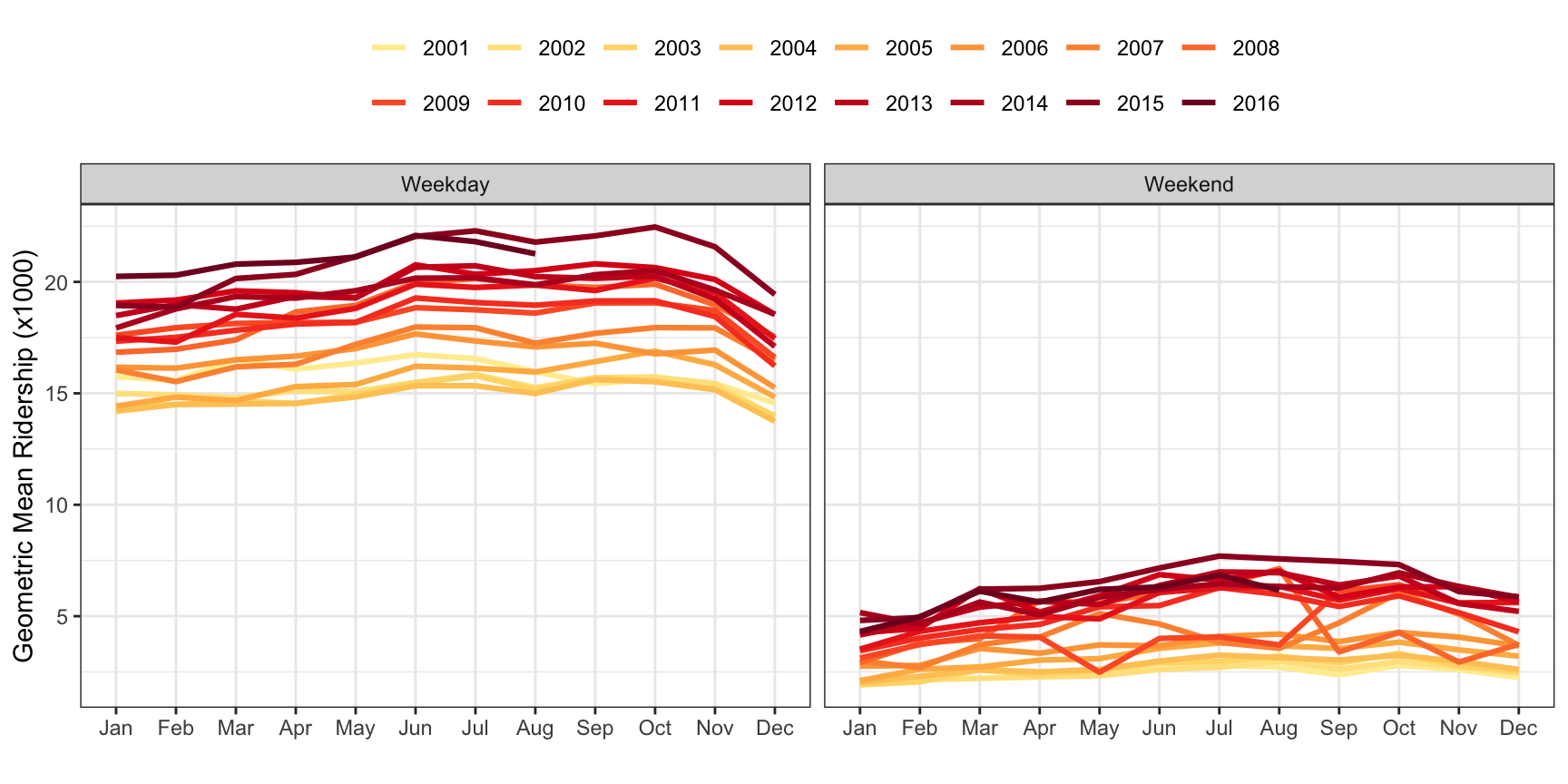
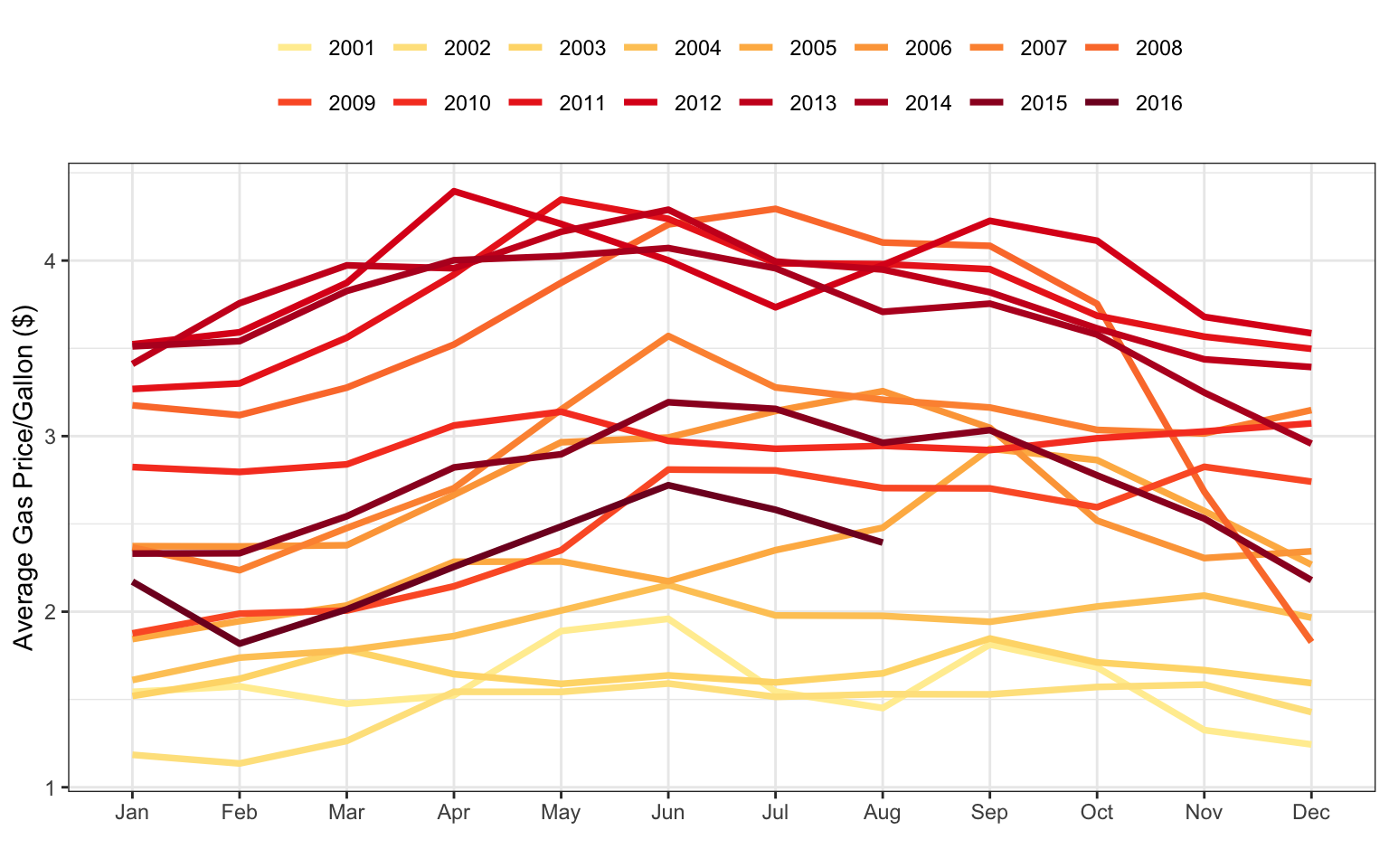
Weekend ridership also shows annual trends but exhibits more variation within the trends for some years. Uncovering predictors associated with this increased variation could help reduce forecasting error. Specifically, the Weekend line plots have the highest variation during 2008, with much higher ridership in the summer. A potential driver for increased ridership on public transportation is gasoline prices. Weekly gas prices in the Chicago area were collected from the U.S. Energy Information Administration, and the monthly average price by year is shown in the line plot of Figure 4.10.
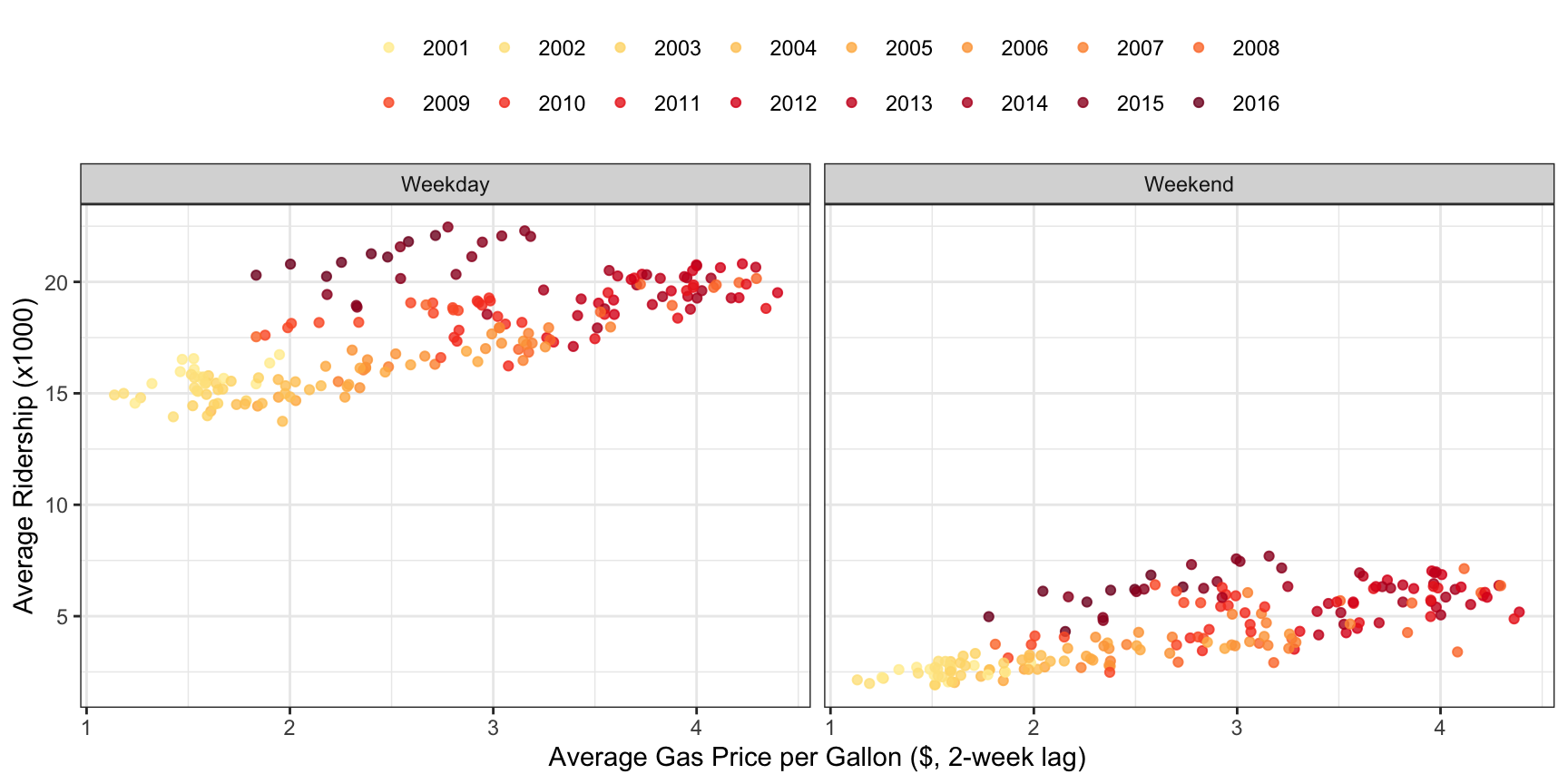
Next, let’s see if a relationship can be established between gas prices and ridership. To do this, we will calculate the monthly average 2-week lag in gas price and the geometric mean of ridership at the Clark/Lake station. Figure 4.11 illustrates this relationship; there is a positive association between the 2-week lag in gas price and the geometric mean of ridership. From 2001 through 2014, the higher the gas price, the higher the ridership, with 2008 data appearing at the far right of both the Weekday and Weekend scatter plots. This trend is slightly different for 2015 and 2016 when oil prices dropped due to a marked increase in supply (U.S. Energy Information Administration 2017b). Here we see that by digging in to characteristics of the original line plot, another feature can be found that will be useful for explaining some of the variation in ridership.
4.2.7 Principal Components Analysis
It is possible to visualize five or six dimensions of data in a two-dimensional figure by using colors, shapes, and faceting. But almost any data set today contains many more than just a handful of variables. Being able to visualize many dimensions in the physical space that we can actually see is crucial to understanding the data and to understanding if there characteristics of the data that point to the need for feature engineering. One way to condense many dimensions into just two or three is to use projection techniques such as principal components analysis (PCA), partial least squares (PLS), or multidimensional scaling (MDS). Dimension reduction techniques for the purpose of feature engineering will be more fully addressed in Section 6.3. Here we will highlight PCA, and how this method can be used to engineer features that effectively condense the original predictors’ information.
Predictors that are highly correlated, like the station ridership illustrated in Figure 4.8, can be thought of as existing in a lower dimensional space than the original data. That is, the data represented here could be approximately represented by combinations of similar stations. Principal components analysis finds combinations of the variables that best summarizes the variability in the original data (Dillon and Goldstein 1984). The combinations are a simpler representation of the data and often identify underlying characteristics within the data that will help guide the feature engineering process.
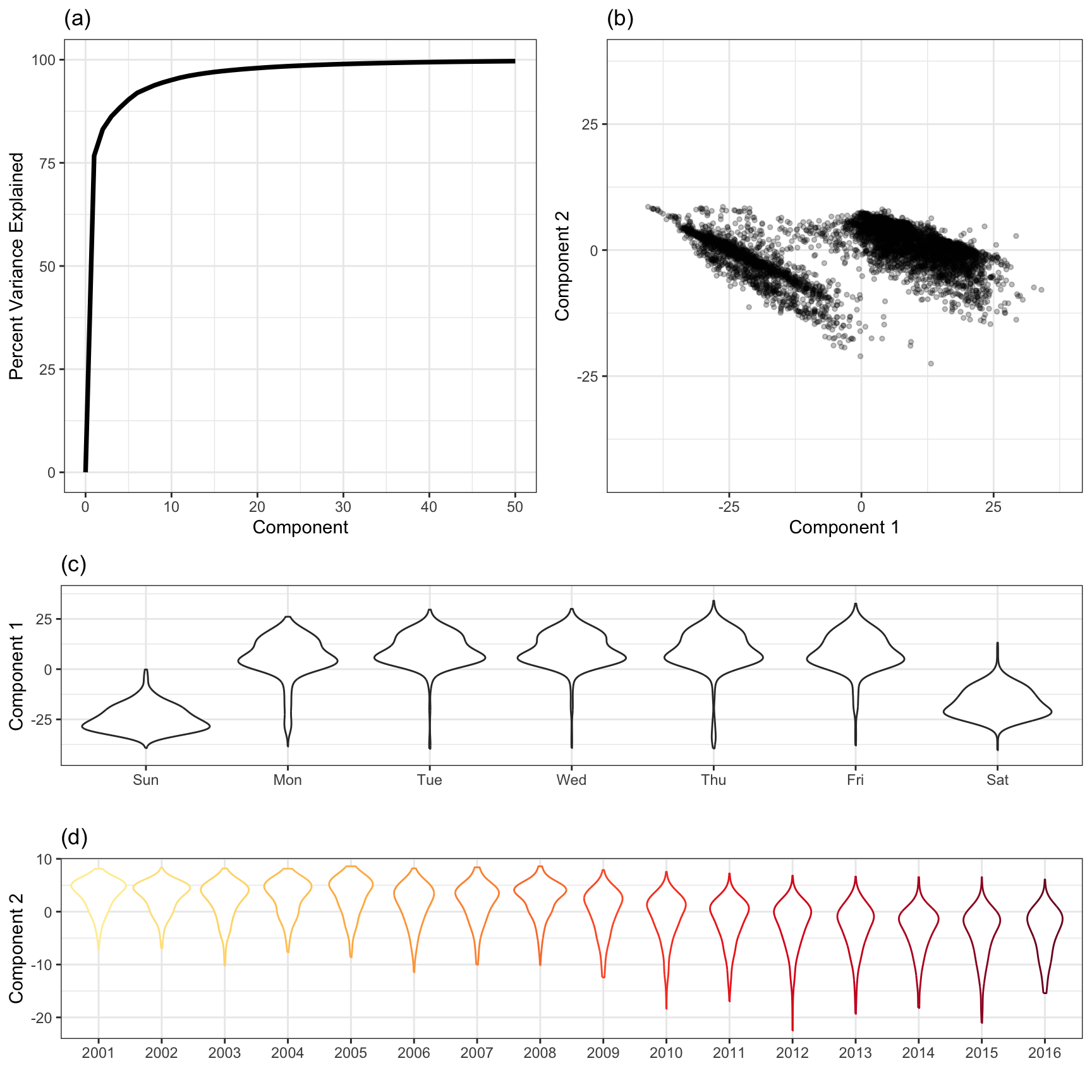
PCA will now be applied to the 14-day lagged station ridership data. Because the objective of PCA is to optimally summarize variability in the data, the cumulative percentage of variation is summarized by the top components. For these data, the first component captures 76.7% of the overall variability, while the first two components capture 83.1%. This is a large percentage of variation given that there are 125 total stations, indicating that station ridership information is redundant and can likely be summarized in a more condensed fashion.
Figure 4.12 provides a summary of the analysis. Part (a) displays the cumulative amount of variation summarized across the first 50 components. This type of plot is used to visually determine how many components are required to summarize a sufficient amount of variation in the data. Examining a scatter plot of the first two components (b) reveals that PCA is focusing on variation due to the part of the week with the weekday samples with lower component 1 scores and weekend samples with higher component 1 scores. The second component focuses on variation due to change over time with earlier samples receiving lower component 2 scores and later samples receiving higher component 2 scores. These patterns are revealed more clearly in parts (c) and (d) where the first and second component are plotted against the underlying variables that appear to affect them the most.
Other visualizations earlier in this chapter already alerted us to the importance of part of the week and year relative to the response. PCA now helps to confirm these findings, and will enable the creation of new features that simplify our data while retaining crucial predictive information. We will delve into this techniques and other similar techniques later in Section 6.3.
4.3 Visualizations for Categorical Data: Exploring the OkCupid Data
To illustrate different visualization techniques for qualitative data, the OkCupid data are used. These data were first introduced in Section 3.1. Recall that the training set consisted of 38,809 profiles and the goal was to predict whether the profile’s author was worked in a STEM field. The event rate is 18.5% and most predictors were categorical in nature. These data are discussed more in the next chapter.
4.3.1 Visualizing Relationships Between Outcomes and Predictors
Traditionally, bar charts are used to represent counts of categorical values. For example, Figure 4.13(a) shows the frequency of the stated religion, partitioned and colored by outcome category. The virtue of this plot is that it is easy to see the most and least frequent categories. However, it is otherwise problematic for several reasons:
To understand if any religions are associated with the outcome, the reader’s task is to visually judge the ratio of each dark blue bar to the corresponding light blue bar across all religions and to then determine if any of the ratios are different from random chance. This figure is ordered from greatest ratio (left) to least ratio (right) which, in this form, may be difficult for the reader see.
The plot is indirectly illustrating the characteristic of data that we are interested in, specifically, the ratio of frequencies between the STEM and non-STEM profiles. We don’t care how many Hindus are in STEM fields; instead, the ratio of fields within the Hindu religion is the focus. In other words, the plot obscures the statistical hypothesis that we are interested in: is the rate of Hindu STEM profiles different than what we would expect by chance?
If the rate of STEM profiles within a religion is the focus, bar charts give no sense of uncertainty in that quantity. In this case, the uncertainty comes from two sources. First, the number of profiles in each religion can obviously affect the variation in the proportion of STEM profiles. This is illustrated by the height of the bars but this isn’t a precise way to illustrate the noise. Second, since the statistic of interest is a proportion, the variability in the statistic becomes larger as the rate of STEM profiles approaches 50% (all other things being equal).
To solve the first two issues, we might show the within-religion percentages of the STEM profiles. Figure 4.13(b) shows this alternative version of the bar chart, which is an improvement since the proportion of STEM profiles is now the focus. It is more obvious how the religions were ordered and we can see how much each deviates from the baseline rate of 18.4%. However, we still haven’t illustrated the uncertainty. Therefore, we cannot assess if the rates for the profiles with no stated religion are truly different from agnostics. Also, while Figure 4.13(b) directly compares proportions across religions, it does not give any sense of the frequency of each religion. For these data there are very few Islamic profiles; this important information cannot be seen in this display.
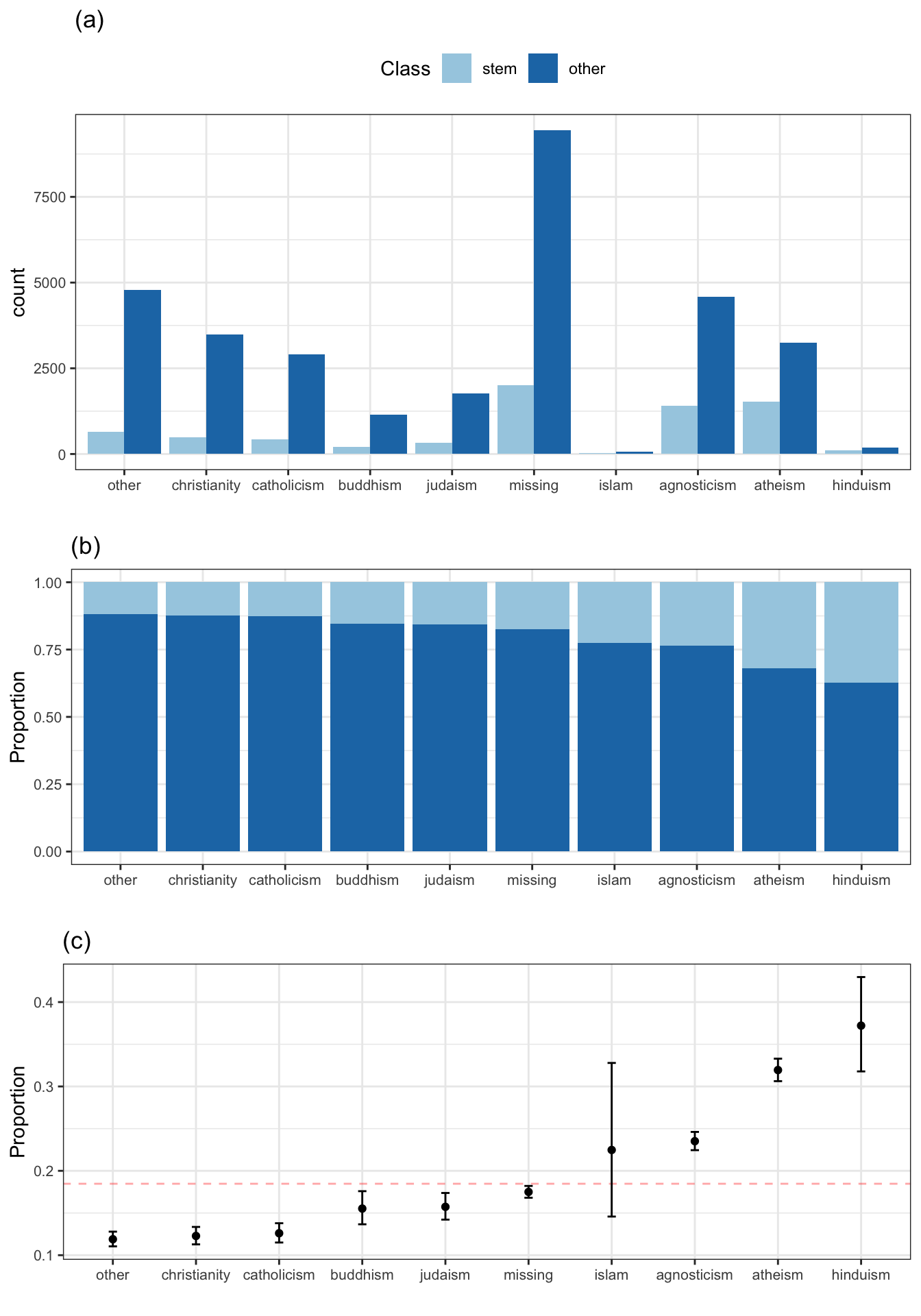
Figure 4.13(c) solves all three of the problems listed above. For each religion, the proportion of STEM profiles is calculated and a 95% confidence interval is shown to help understand what the noise is around this value. We can clearly see which religions deviate from randomness and the width of the error bars help the reader understand how much each number should be trusted. This image is the best of the three since it directly shows the magnitude of the difference as well as the uncertainty. In situations where the number of categories on the x-axis is large, a volcano plot can be used to show the results (see Figures Figure 2.6 and Figure 5.3).
The point of this discussion is not that summary statistics with confidence intervals are always the solution to a visualization problem. The takeaway message is that each graph should have a clearly defined hypothesis and that this hypothesis is shown concisely in a way that allows the reader to make quick and informative judgments based on the data.
Finally, does religion appear to be related to the outcome? Since there is a gradation of rates of STEM professions between the groups, it would appear so. If there were no relationship, all of the rates would be approximately the same.
How would one visualize the relationship between a categorical outcome and a numeric predictor? As an example, total length of all the profile essays will be used to illustrate a possible solution. There were 1181 profiles in the training set where the user did not fill out any of the open text fields. In this analysis, all of the nine answers were concatenated into a single text string The distribution of the text length was very left-skewed with a median value of 1,862 characters. The maximum length was approximately 59K characters although 10% of the profiles contained less than 444 characters. To investigate this, the distribution of the total number of essay characters is shown in Figure 4.14(a). The x-axis is the log of the character count and profiles without essay text are shown here as a zero. The distributions appear to be extremely similar between classes so this predictor (in isolation) is unlikely to be important by itself. However, as discussed above, it would be better to try to directly answer the question.
To do this, another smoother is used to model the data. In this case, a regression spline smoother (Wood 2006) is used to model the probability of a STEM profile as a function of the (log) essay length. This involves fitting a logistic regression model using a basis expansion. This means that our original factor, log essay length, is used to create a set of artificial features that will go into a logistic regression model. The nature of these predictors will allow a flexible, local representation of the class probability across values of essay length and are discussed more in Section 6.2.16.
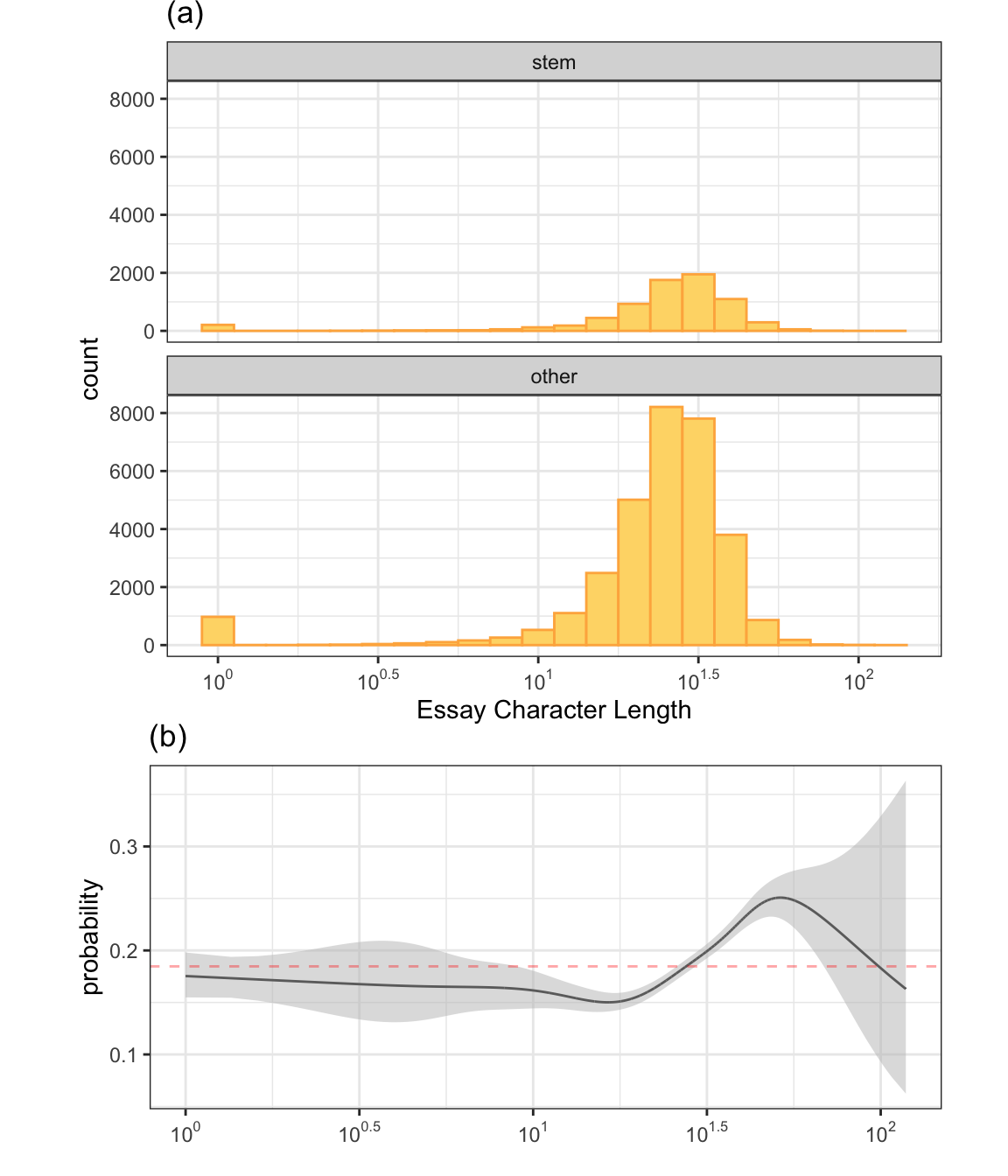
The results are shown in Figure 4.14(b). The black line represents the class probability of the logistic regression model and the bands denote 95% confidence intervals around the fit. The horizontal red line indicates the baseline probability of STEM profiles from the training set. Prior to a length of about \(10^{1.5}\), the profile is slightly less likely than chance to be STEM. Larger profiles show and increase in the probability. This might seem like a worthwhile predictor but consider the scale of the y-axis. If this were put in the full probability scale of [0, 1], the trend would appear virtually flat. At most, the increase in the likelihood of being a STEM profile is almost 3.5%. Also, note that the confidence bands rapidly expand around \(10^{1.75}\) mostly due to a decreasing number of data points in this range so the potential increase in probability has a high degree of uncertainty. This predictor might be worth including in a model but is unlikely to show a strong effect on its own.
4.3.2 Exploring Relationships Between Categorical Predictors
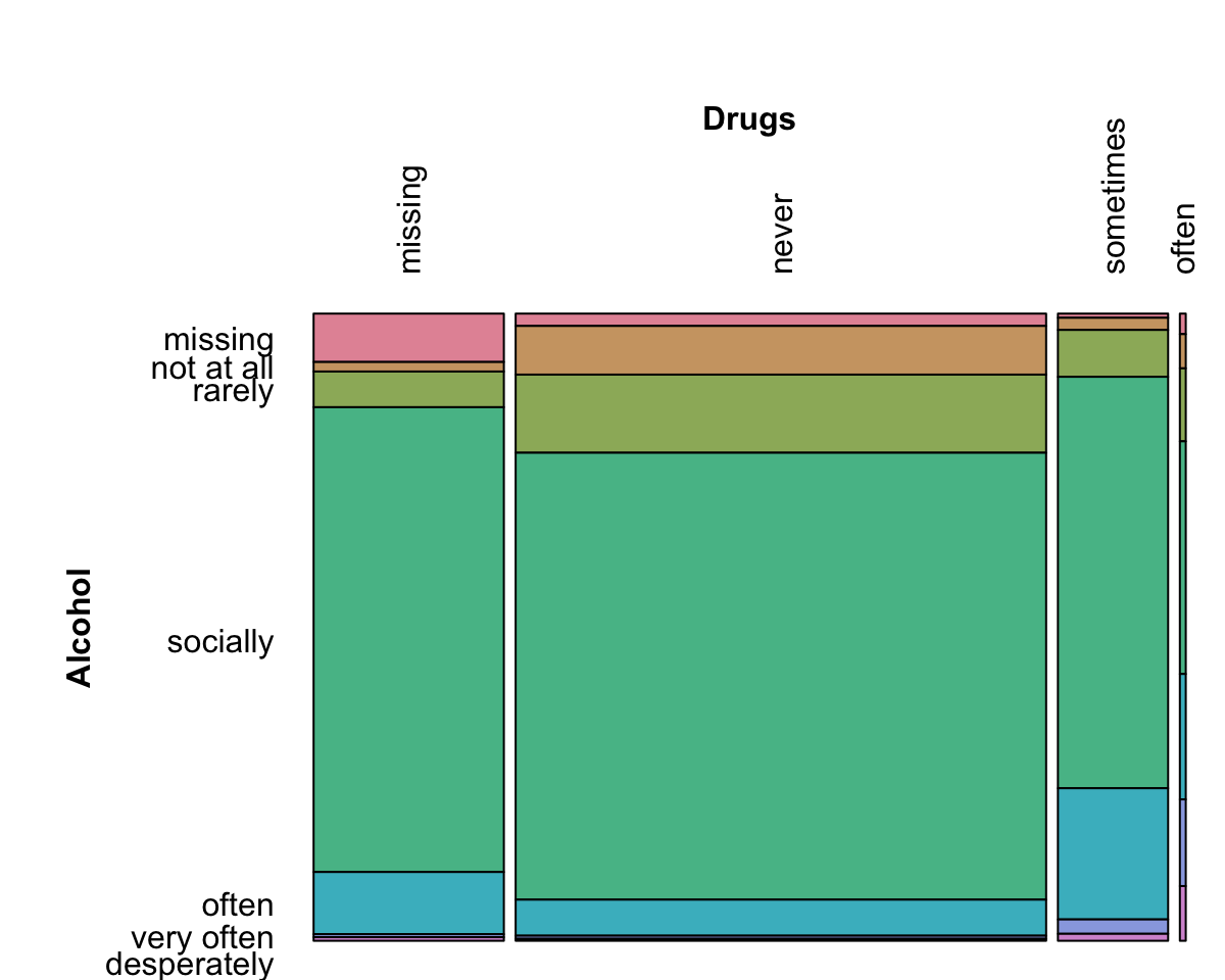
Before deciding how to use predictors that contain non-numeric data, it is critical to understand their characteristics and relationships with other predictors. The unfortunate practice that is often seen relies on a large number of basic statistical analyses of two-way tables that boil relationships down to numerical summaries such as the Chi-squared (\(\chi^2\)) test of association. Often the best approach is to visualize the data. When considering relationships between categorical data, there are several options. Once a cross-tabulation between variables is created, mosaic plots can once again be used to understand the relationship between variables. For the OkCupid data, it is conceivable that the questionnaires for drug and alcohol use might be related and, for these variables, Figure 4.15 shows the mosaic plot. For alcohol, the majority of the data indicate social drinking while the vast majority of the drug responses were “never” or missing. Is there any relationship between these variables? Do any of the responses “cluster” with others?
These questions can be answered using correspondence analysis (Greenacre 2017) where the cross-tabulation is analyzed. In a contingency table, the frequency distributions of the variables can be used to determine the expected cell counts which mimic what would occur if the two variables had no relationship. The traditional \(\chi^2\) test uses the deviations from these expected values to assess the association between the variables by adding up functions of this type of cell residuals. If the two variables in the table are strongly associated, the overall \(\chi^2\) statistic is large. Instead of summing up these residual functions, correspondence analysis analyzes them to determine new variables that account for the largest fraction of these statistics7. These new variables, called the principal coordinates, can be computed for both variables in the table and shown in the same plot. These plots can contain several features:
The data on each axis would be evaluated in terms of how much of the information in the original table that the principal coordinate accounts for. If a coordinate only captures a small percentage of the overall \(\chi^2\) statistic, the patterns shown in that direction should not be over-interpreted.
Categories that fall near the origin represent the “average” value of the data From the mosaic plot, it is clear that there are categories for each variable that have the largest cell frequencies (e.g., “never” drugs and “social” alcohol consumption). More unusual categories are located on the outskirts of the principal coordinate scatter plot.
Categories for a single variable whose principal coordinates are close to one another are indicative of redundancy, meaning that there may be the possibility of pooling these groups.
Categories in different variables that fall near each other in the principal coordinate space indicate an association between these categories.
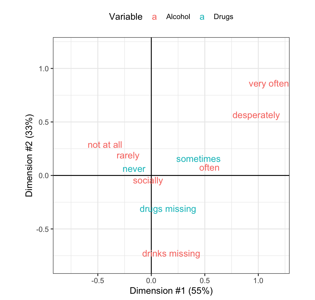
In the cross-tabulation between alcohol and drug use, the \(\chi^2\) statistic is very large (4114.2) for its degrees of freedom (18) and is associated with a very small p-value (0). This indicates that there is a strong association between these two variables.
Figure 4.16 shows the principal coordinates from the correspondence analysis. The component on the x-axis accounts for more than half of the \(\chi^2\) statistics. The values around zero in this dimension tends to indicate that no choice was made or sporadic substance use. To the right, away from zero, are less frequently occurring values. A small cluster indicates that occasional drug use and frequent drinking tend to have a specific association in the data. Another, more extreme, cluster shows that using alcohol very often and drugs have an association. The y-axis of the plot is mostly driven by the missing data (understandably since 25.8% of the table has at least one missing response) and accounts for another third of the \(\chi^2\) statistics. These results indicate that these two variables have similar results and might be measuring the same underlying characteristic.
4.4 Post Modeling Exploratory Visualizations
As previously mentioned in Section 3.2.2, predictions on the assessment data produced during resampling can be used to understand performance of a model. It can also guide the modeler to understand the next set of improvements that could be made using visualization and analysis. Here, this process is illustrated using the train ridership data.
Multiple linear regression has a rich set of diagnostics based on model residuals that aid in understanding the model fit and in identifying relationships that may be useful to include in the model. While multiple linear regression lags in predictive performance to other modeling techniques, the available diagnostics are magnificent tools that should not be underestimated in uncovering predictors and predictor relationships that can benefit more complex modeling techniques.
One tool from regression diagnosis that is helpful for identifying useful predictors is the partial regression plot (Neter et al. 1996). This plot utilizes residuals from two distinct linear regression models to unearth the potential usefulness of a predictor in a model. To begin the process, we start by fitting the following model and computing the residuals (\(\epsilon_i\)):
\[ y_i = \beta_1 x_1 + \beta_2 x_2 + \cdots + \beta_p x_p + \epsilon_i \] Next, we select a predictor that was not in the model, but may contain additional predictive information with respect to the response. For the potential predictor, we then fit:
\[ x_{new_i} = \beta_1 x_1 + \beta_2 x_2 + \cdots + \beta_p x_p + \eta_i \] The residuals (\(\epsilon_i\) and \(\eta_i\)) from the models are then plotted against each other in a simple scatter plot. A linear or curvi-linear pattern between these sets of residuals are an indication that the new predictor as a linear or quadratic (or some other non-linear variant) term would be a useful addition in the model.
As previously mentioned, it is problematic to examine the model fit via residuals when those values are determined by simply pre-predicting the training set data. A better strategy is to use the residuals from the various assessment sets created during resampling.
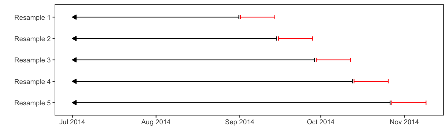
For the Chicago data, a rolling forecast origin scheme (Section 3.4.4) was used for resampling. There are 5698 data points in the training set, each representing a single day. The resampling used here contains a base set of samples before September 01, 2014 and the analysis/assessment splits begins at this date. In doing this, the analysis set grows cumulatively; once an assessment set is evaluated, it is put into the analysis set on the next iteration of resampling. Each assessment set contains the 14 days immediately after the last value in the analysis set. As a result, there are 52 resamples and each assessment set is a mutually exclusive collection of the latest dates. This scheme is meant to mimic how the data would be repeatedly analyzed; once a new set of data are captured, the previous set is used to train the model and the new data are used as a test set. Figure 4.17 shows an illustration of the first few resamples. The arrows on the left-hand side indicate that the full analysis set starts on January 22, 2001.
For any model fit to these data using such a scheme, the collection of 14 sets of residuals can be used to understand the strengths and weaknesses of the model with minimal risk of overfitting. Also, since the assessment sets move over blocks of time, it also allows the analyst to understand if there are any specific times of year that the model does poorly.
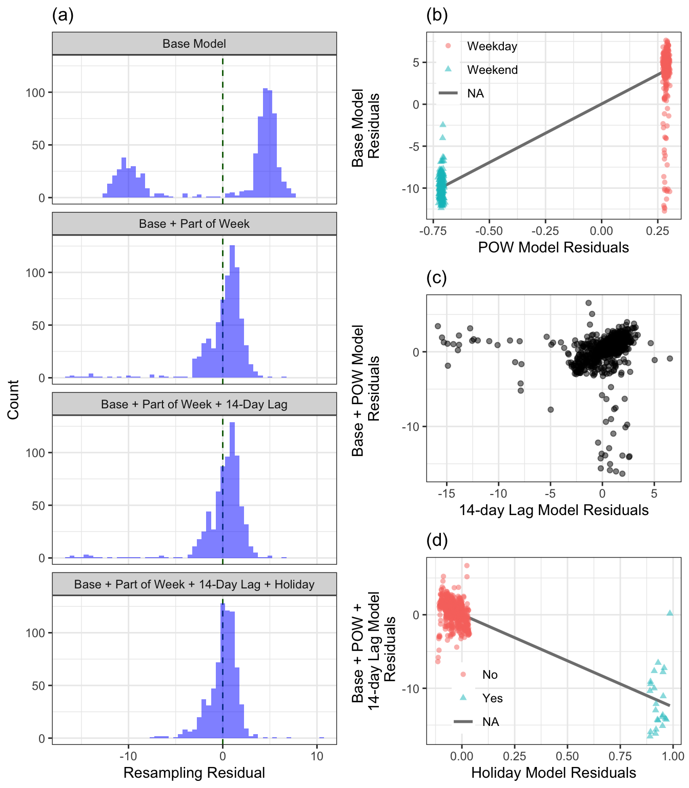
The response for the regression model is the ridership at the Clark/Lake station, and our initial model will contain the predictors of week, month and year. The distribution of the hold-out residuals from this model are provided in Figure 4.18(a). As we saw earlier in this chapter, the distribution has two peaks, which we found were due to the part of the week (weekday versus weekend). To investigate the importance of part of the week we then regress the base predictors on part of the week and compute the hold-out residuals from this model. The relationship between sets of hold-out residuals is provided in (b) which demonstrates the non-random relationship, indicating that part of the week contains additional predictive information for the Clark/Lake station ridership. We can see that including part of the week in the model further reduces the residual distribution as illustrated in the histogram labeled Base + Part of Week.
Next, let’s explore the importance of the 14-day lag of ridership at the Clark/Lake station. Part (c) of the figure demonstrates the importance of including the 14-day lag of ridership at the Clark/Lake station. In this part of the figure we see a strong linear relationship between the model residuals in the mainstream of the data, with a handful of days lying outside of the overall pattern. These days happen to be holidays for this time period. The potential predictive importance of holidays are reflected in part (d). In this figure, the reader’s eye may be drawn to one holiday that lies far away from the rest of the holiday samples. It turns out that this sample is July 4, 2015, and is the only day in the training data that is both a holiday and weekend day. Because the model already accounted for part of the week, this additional information that this day is a holiday has virtually no effect on the predicted value for this sample.
4.5 Summary
Advanced predictive modeling and machine learning techniques offer the allure of being able to extract complex relationships between predictors and the response with little effort by the analyst. This hands-off approach to modeling will only put the analyst at a disadvantage. Spending time visualizing the response, predictors, relationships among the predictors, and relationships between predictors and the response can only lead to better understandings of the data. Moreover, this knowledge may provide crucial insights as to what features may be missing in the data and may need to be included to improve a model’s predictive performance.
Data visualization is a foundational tool of feature engineering. The next chapter uses this base and begins the development of feature engineering for categorical predictors.
4.6 Computing
The website http://bit.ly/fes-eda contains R programs for reproducing these analyses.
Chapter References
Cleveland, W. 1979. “Robust Locally Weighted Regression and Smoothing Scatterplots.” Journal of the American Statistical Association 74 (368): 829–36.
Cleveland, W. 1993. Visualizing Data. Summit, New Jersey: Hobart Press.
Dillon, W, and M Goldstein. 1984. Multivariate Analysis Methods and Applications. Wiley.
Frigge, M, D Hoaglin, and B Iglewicz. 1989. “Some Implementations of the Boxplot.” The American Statistician 43 (1): 50–54.
Greenacre, M. 2017. Correspondence Analysis in Practice. CRC press.
Healy, K. 2018. Data Visualization: A Practical Introduction. Princeton University Press.
Hintze, J, and R Nelson. 1998. “Violin Plots: A Box Plot-Density Trace Synergism.” The American Statistician 52 (2): 181–84.
Neter, J, M Kutner, C Nachtsheim, and W Wasserman. 1996. Applied Linear Statistical Models. Irwin Chicago.
Tufte, E. 1990. Envisioning Information. Cheshire, Connecticut: Graphics Press.
Tukey, John W. 1977. Exploratory Data Analysis. Reading, Mass.
United States Census Bureau. 2017. “Chicago Illinois Population Estimates.” https://tinyurl.com/y8s2y4bh.
U.S. Energy Information Administration. 2017a. “Weekly Chicago All Grades All Formulations Retail Gasoline Prices.” https://tinyurl.com/ydctltn4.
U.S. Energy Information Administration. 2017b. “What Drives Crude Oil Prices?” https://tinyurl.com/supply-opec.
Wood, S. 2006. Generalized Additive Models: An Introduction with r. Chapman; Hall/CRC.
The stations selected contained no missing values. See Section 8.5 for more details.↩︎
Another alternative would be to simply compute the daily average values for these conditions from the entire training set.↩︎
This visualization approach is also referred to as “trellising” or “conditioning” in different software.↩︎
This does lead to an interesting dilemma for this analysis: should such an aberrant instance be allowed to potentially influence the model? We have left the value untouched but a strong case could be made for imputing what the value would be from previous data and using this value in the analysis.↩︎
There are other types of smoothers that can be used to discover potential nonlinear patterns in the data. One, called
loess, is very effective and uses a series of moving regression lines across the predictor values to make predictions at a particular point (Cleveland 1979).↩︎The mechanisms are very similar to principal component analysis (PCA), discussed in Chapter 6. For example, both use a singular value decomposition to compute the new variables.↩︎