11 Greedy Search Methods
In this chapter, greedy search methods such as simple univariate filters and recursive feature elimination are discussed. Before proceeding, another data set is introduced that will be used in this chapter to demonstrate the strengths and weaknesses of these approaches.
11.1 Illustrative Data: Predicting Parkinson’s Disease
Sakar et al. (2019) describes an experiment where a group of 252 patients, 188 of whom had a previous diagnosis of Parkinson’s disease, were recorded speaking a particular sound three separate times. Several signal processing techniques were then applied to each replicate to create 750 numerical features. The objective was to use the features to classify patients’ Parkinson’s disease status. Groups of features within these data could be considered as following a profile (Chapter 9), since many of the features consisted of related sets of fields produced by each type of signal processor (e.g., across different sound wavelengths or sub-bands). Not surprisingly, the resulting data have extreme amount of multicollinearity; about 10,750 pairs of predictors have absolute rank correlations greater than 0.75.
Since each patient had three replicated data points, the feature results used in our analyses are the averages of the replicates. In this way, the patient is both the independent experimental unit and the unit of prediction.
To illustrate the tools in this chapter, we used a stratified random sample based on patient disease status to allocate 25% of the data to the test set. The resulting training set consisted of 189 patients, 138 of whom had the disease. The performance metric to evaluate models was the area under the ROC curve.
11.2 Simple Filters
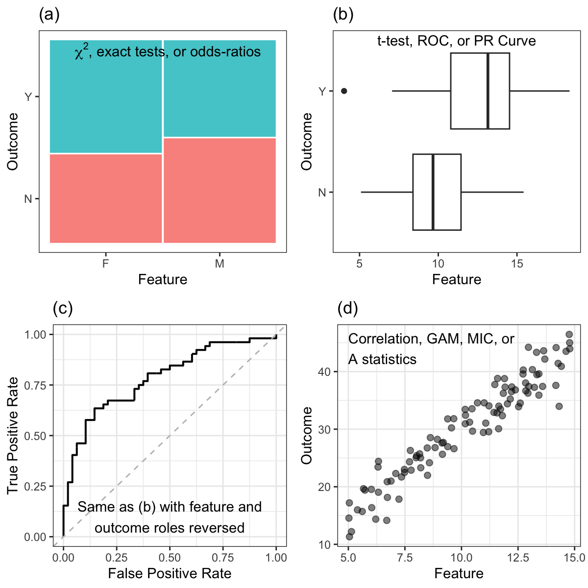
The most basic approach to feature selection is to screen the predictors to see if any have a relationship with the outcome prior to including them in a model. To do this, a numeric scoring technique is required to quantify the strength of the relationship. Using the scores, the predictors are ranked and filtered with either a threshold or by taking the top \(p\) predictors. Scoring the predictors can be done separately for each predictor, or can be done simultaneously across all predictors (depending on the technique that is used). If the predictors are screened separately, there are a large variety of scoring methods. A summary of some popular and effective scoring techniques are provided below and are organized based on the type of predictor and outcome. The list is not meant to be exhaustive, but is meant to be a starting place. A similar discussion in contained in Chapter 18 of Kuhn and Johnson (2013).
When screening individual categorical predictors, there are several options depending on the type of outcome data:
When the outcome is categorical, the relationship between the predictor and outcome forms a contingency table. When there are three or more levels for the predictor, the degree of association between predictor and outcome can be measured with statistics such as \(\chi^2\) (chi-squared) tests or exact methods (Agresti 2012). When there are exactly two classes for the predictor, the odds-ratio can be an effective choice (see Section 5.6).
When the outcome is numeric, and the categorical predictor has two levels, then a basic \(t\)-test can be used to generate a statistic. ROC curves and precision-recall curves can also be created for each predictor and the area under the curves can be calculated1. When the predictor has more than two levels, the traditional ANOVA \(F\)-statistic can be calculated.
When the predictor is numeric, the following options exist:
When the outcome is categorical, the same tests can be used in the case above where the predictor is categorical and the outcome is numeric. The roles are simply reversed in the t-test, curve calculations, \(F\)-test, and so on. When there are a large number of tests or if the predictors have substantial multicollinearity, the correlation-adjusted t-scores of Opgen-Rhein and Strimmer (2007) and Zuber and Strimmer (2009) are a good alternative to simple ANOVA statistics.
When the outcome is numeric, a simple pairwise correlation (or rank correlation) statistic can be calculated. If the relationship is nonlinear, then the maximal information coefficient (MIC) values (Reshef et al. 2011) or \(A\) statistics (Murrell, Murrell, and Murrell 2016), which measure strength of the association between numeric outcomes and predictors, can be used.
Alternatively, a generalized additive model (GAM) (Wood 2006) can fit nonlinear smooth terms to a set of predictors simultaneously and measure their importance using a p-value that tests against a null hypothesis that there is no trend of each predictor. An example of such a model with a categorical outcome was shown in Figure 4.14(b).
A summary of these simple filters can be found in Figure 11.1.
Generating summaries of how effective individual predictors are at classifying or correlating with the outcome is straightforward when the predictors are all of the same type. But most data sets contain a mix of predictor types. In this setting it can be challenging to arrive at a ranking of the predictors since their screening statistics are in different units. For example, an odds-ratio and a t-statistic are not compatible since they are on different scales. In many cases, each statistic can be converted to a p-value so that there is a commonality across the screening statistics.
Recall that a p-value stems from the statistical framework of hypothesis testing. In this framework, we assume that there is no association between the predictor and the outcome. The data are then used to refute the assumption of no association. The p-value is then the probability that we observe a more extreme value of the statistic if, in fact, no association exists between the predictor and outcome.
Each statistic can be converted to a p-value, but this conversion is easier for some statistics than others. For instance, converting a \(t\)-statistic to a p-value is a well-known process, provided that some basic assumptions are true. On the other hand, it is not easy to convert an AUC to a p-value. A solution to this problem is by using a permutation method (Good 2013; Berry, Mielke Jr, and Johnston 2016). This approach can be applied to any statistic to generate a p-value. Here is how a randomization approach works: for a selected predictor and corresponding outcome, the predictor is randomly permuted, but the outcome is not. The statistic of interest is then calculated on the permuted data. This process disconnects the observed predictor and outcome relationship, thus creating no association between the two. The same predictor is randomly permuted many times to generate a distribution of statistics. This distribution represents the distribution of no association (i.e., the null distribution). The statistic from the original data can then be compared to the distribution of no association to get a probability, or p-value, of coming from this distribution. An example of this is given in Kuhn and Johnson (2013) for Relief scores (Robnik-Sikonja and Kononenko 2003).
In March of 2016, the American Statistical Association released a statement2 regarding the use of p-values (and null-hypothesis-based test) to discuss their utility and misuse. For example, one obvious issue is the application of a arbitrarily defined threshold to determine “significant” outside of any practical context can be problematic. Also, it is important to realize when a statistic such as the area under the ROC curve is converted into a p-value, the level of evidence required for “importance” is being set very low. The reason for this is that the null hypothesis is no association. One might think that, if feature A has a p-value of 0.01 and feature B has a p-value of 0.0001, that the original ROC value was larger for B. This may not be the case since the p-value is a function of signal, noise, and other factors (e.g., the sample size). This is especially true when the p-values are being generated from different data sets; in these cases, the sample size may be the prime determinant of the value.
For our purposes, the p-values are being used algorithmically to search for appropriate subsets, especially since it is a convenient quantity to use when dealing with different predictor types and/or importance statistics. As mentioned in Section 5.6 and below in Section 11.4, it is very important to not take p-values generated in such processes as meaningful or formal indicators of statistical significance.
Good summaries of the issues are contained in Yaddanapudi (2016), Wasserstein and Lazar (2016), and the entirety of Volume 73 of The American Statistician.
Simple filters are effective at identifying individual predictors that are associated with the outcome. However, these filters are very susceptible to finding predictors that have strong associations in the available data but do not show any association with new data. In the statistical literature, these selected predictors are labeled as false positives. An entire sub-field of statistics has been devoted to developing approaches for minimizing the chance of false positive findings, especially in the context of hypothesis testing and p-values. One approach to reducing false positives is to adjust the p-values to effectively make them larger and thus less significant (as was shown in previous chapters).
In the context of predictive modeling, false positive findings can be minimized by using an independent set of data to evaluate the selected features. This context is exactly parallel to the context of identifying optimal model tuning parameters. Recall from Section 3.4 that cross-validation is used to identify an optimal set of tuning parameters such that the model does not overfit the available data. The model building process now needs to accomplish two objectives: to identify an effective subset of features, and to identify the appropriate tuning parameters such that the selected features and tuning parameters do not overfit the available data. When using simple screening filters, selecting both the subset of features and model tuning parameters cannot be done in the same layer of cross-validation, since the filtering must be done independently of the model tuning. Instead, we must incorporate another layer of cross-validation. The first layer, or external layer, is used to filter features. Then the second layer (the “internal layer”) is used to select tuning parameters. A diagram of this process is illustrated in Figure 11.2.

As one can see from this figure, conducting feature selection can be computationally costly. In general, the number of models constructed and evaluated is \(I\times E \times T\), where \(I\) is the number if internal resamples, \(E\) is the number of external resamples, and \(T\) is the total number of tuning parameter combinations.
11.2.1 Simple Filters Applied to the Parkinson’s Disease Data
The Parkinson’s disease data has several characteristics that could make modeling challenging. Specifically, the predictors have a high degree of multicollinearity, the sample size is small, and the outcome is imbalanced (74.6% of patients have the disease). Given these characteristics, partial least squares discriminant analysis (PLSDA, Barker and Rayens (2003)) would be a good first model to try. This model produces linear class boundaries which may constrain it from overfitting to the majority class. The model tuning parameters for PLSDA is the number of components to retain.
The second choice we must make is the criteria for filtering features. For these data we will use the area under the ROC curve to determine if a feature should be included in the model. The initial analysis of the training set showed that there were 5 predictors with an area under the ROC curve of at least 0.80 and 21 were between 0.75 and 0.80.
For the internal resampling process, an audio feature was selected if it had an area under the ROC curve of at least 0.80. The selected features within the internal resampling node are then passed to the corresponding external sampling node where the model tuning process is conducted.
Once the filtering criteria and model are selected, then the type of internal and external resampling methods are chosen. In this example, we used 20 iterations of bootstrap resampling for internal resampling and 5 repeats of 10-fold cross-validation for external resampling. The final estimates of performance are based on the external resampling hold-out sets. To preprocess the data, a Yeo-Johnson transformation was applied to each predictor, then the values were centered and scaled. These operations were conducted within the resampling process.
During resampling the number of predictors selected ranged from 2 to 12 with an average of 5.7. Some predictors were selected regularly; 2 of them passed the ROC threshold in each resample. For the final model, the previously mentioned 5 predictors were selected. For this set of predictors, the PLSDA model was optimized with 4 components. The corresponding estimated area under the ROC curve was 0.827.
Looking at the selected predictors more closely, there appears to be considerable redundancy. Figure 11.3 shows the rank correlation matrix of these predictors in a heatmap. There are very few pairs with absolute correlations less than 0.5 and many extreme values. As mentioned in Section 6.3, partial least squares models are good at feature extraction by creating new variables that are linear combinations of the original data. For this model, these PLS components are created in a way that summarizes the maximum amount of variation in the predictors while simultaneously minimizing the misclassification among groups. The final model used 4 components, each of which is a combination of 5 of the original predictors that survived the filter. Looking at Figure 11.3, there is a relatively clean separation into distinct blocks/clusters. This indicates that there are probably only a handful of underlying pieces of information in the filtered predictors. A separate principal component analysis was used to gauge the magnitude of the between-predictor correlations. In this analysis, only 1 feature was needed to capture 90% of the total variation. This reinforces that there are only small number of underlying effects in these predictors. This is the reason that such a small number of components were found to be optimal.
Did this filtering process help the model? If the same resamples are used to fit the PLS model using the entire predictor set, the model still favored a small number of projections (4 components) and the area under the ROC curve was estimated to be a little better than the full model (0.812 versus 0.827 when filtered). The p-value from a paired t-test (\(p = 0.4465\)) showed no evidence that the improvement is real. However, given that only 0.7% of the original variables were used in this analysis, the simplicity of the new model might be very attractive.
One post hoc analysis that is advisable when conducting feature selection is to determine if the particular subset that is found is any better than a random subset of the same size. To do this, 100 random subsets of 5 predictors were created and PLS models were fitted with the same external cross-validation routine. Where does our specific subset fit within the distribution of performance that we see from a random subset? The area under the ROC curve using the above approach (0.827) was better than 97 percent of the values generated using random subsets of the same size. The largest AUC from a random subset was 0.832. This result grants confidence that the filtering and modeling approach found a subset with credible signal. However, given the amount of correlation between the predictors, it is unlikely that this is the only subset of this size that could achieve equal performance.
While partial least squares is very proficient at accommodating predictor sets with a high degree of collinearity, it does raise the question about what the minimal variable set might be that would achieve nearly optimal predictive performance. For this example, we could reduce the subset size by increasing the stringency of the filter (i.e., \(AUC > 0.80\)). Changing the threshold will affect both the sparsity of the solution and the performance of the model. This process is the same as backwards selection which will be discussed in the next section.
To summarize, the use of a simple screen prior to modeling can be effective and relatively efficient. The filters should be included in the resampling process to avoid optimistic assessments of performance. The drawback is that there may be some redundancy in the selected features and the subjectivity around the filtering threshold might leave the modeler wanting to understand how many features could be removed before performance is impacted.
11.3 Recursive Feature Elimination
As previously noted, recursive feature elimination (RFE, Guyon et al. (2002)) is basically a backward selection of the predictors. This technique begins by building a model on the entire set of predictors and computing an importance score for each predictor. The least important predictor(s) are then removed, the model is re-built, and importance scores are computed again. In practice, the analyst specifies the number of predictor subsets to evaluate as well as each subset’s size. Therefore, the subset size is a tuning parameter for RFE. The subset size that optimizes the performance criteria is used to select the predictors based on the importance rankings. The optimal subset is then used to train the final model.
Section 10.4 described in detail the appropriate way to estimate the subset size. The selection process is resampled in the same way as fundamental tuning parameters from a model, such as the number of nearest neighbors or the amount of weight decay in a neural network. The resampling process includes the feature selection routine and the external resamples are used to estimate the appropriate subset size.
Not all models can be paired with the RFE method, and some models benefit more from RFE than others. Because RFE requires that the initial model uses the full predictor set, some models cannot be used when the number of predictors exceeds the number of samples. As noted in previous chapters, these models include multiple linear regression, logistic regression, and linear discriminant analysis. If we desire to use one of these techniques with RFE, then the predictors must first be winnowed down. In addition, some models benefit more from the use of RFE than others. Random forest is one such case (Svetnik et al. 2003) and RFE will be demonstrated using this model for the Parkinson’s disease data.
Backwards selection is frequently used with random forest models for two reasons. First, as noted in Chapter 10, random forest tends not to exclude variables from the prediction equation. The reason is related to the nature of model ensembles. Increased performance in ensembles is related to the diversity in the constituent models; averaging models that are effectively the same does not drive down the variation in the model predictions. For this reason, random forest coerces the trees to contain sub-optimal splits of the predictors using a random sample of predictors3. The act of restricting the number of predictors that could possibly be used in a split increases the likelihood that an irrelevant predictor will be chosen. While such a predictor may not have much direct impact on the performance of the model, the prediction equation is functionally dependent on that predictor. As our simulations showed, tree ensembles may use every possible predictor at least once in the ensemble. For this reason, random forest can use some post hoc pruning of variables that are not essential for the model to perform well. When many irrelevant predictors are included in the data and the RFE process is paired with random forest, a wide range of subset sizes can exhibit very similar predictive performances.
The second reason that random forest is used with RFE is because this model has a well-known internal method for measuring feature importance. This was described previously in Section 7.4 and can be used with the first model fit within RFE, where the entire predictor set is used to compute the feature rankings.
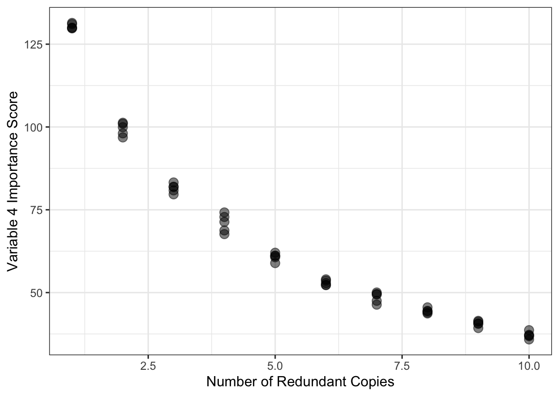
One notable issue with measuring importance in trees is related to multicollinearity. If there are highly correlated predictors in a training set that are useful for predicting the outcome, then which predictor is chosen is essentially a random selection. It is common to see that a set of highly redundant and useful predictors are all used in the splits across the ensemble of trees. In this scenario, the predictive performance of the ensemble of trees is unaffected by highly correlated, useful features. However, the redundancy of the features dilutes the importance scores. Figure 11.4 shows an example of this phenomenon. The data were simulated using the same system described in Section 10.3 and a random forest model was tuned using 2,000 trees. The largest importance was associated with feature \(x_4\). Additional copies of this feature were added to the data set and the model was refit. The figure shows the decrease in importance for \(x_4\) as copies are added4. There is a clear decrease in importance as redundant features are added to the model. For this reason, we should be careful about labeling predictors as unimportant when their permutation scores are not large since these may be masked by correlated variables. When using RFE with random forest, or other tree-based models, we advise experimenting with filtering out highly correlated features prior to beginning the routine.
For the Parkinson’s data, backwards selection was conducted with random forests,5 and each ensemble contained 10,000 trees6. The model’s importance scores were used to rank the predictors. Given the number of predictors and the large amount of correlation between them, the subset sizes were specified on the \(\log_{10}\) scale so that the models would more thoroughly investigate smaller sizes. The same resampling scheme was used as the simple filtering analysis.
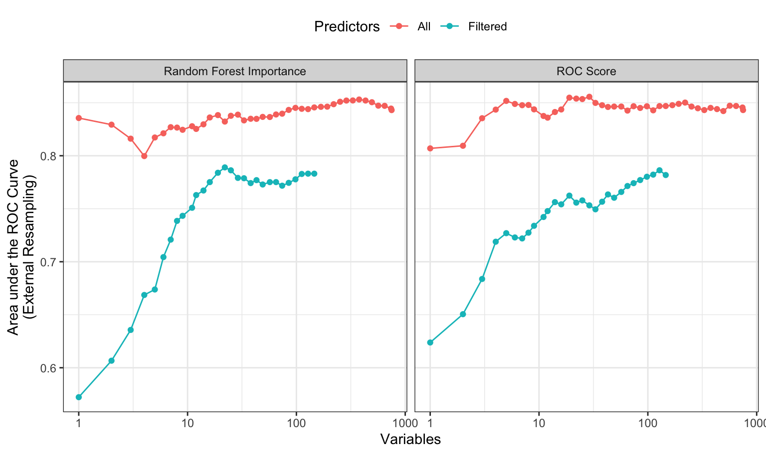
Given our previous comments regarding correlated predictors, the RFE analysis was conducted with and without a correlation filter that excluded enough predictors to coerce all of the absolute pairwise correlations to be smaller than 0.50. The performance profiles, shown in the left-hand panel of Figure 11.5, illustrates that the models created using all predictors show an edge in model performance; the ROC curve AUC was 0.064 larger with a confidence interval for the difference being (0.037, 0.091). Both curves show a fairly typical pattern; performance stays fairly constant until relevant features are removed. Based on the unfiltered models, the numerically best subset size is 377 predictors, although the filtered model could probably achieve similar performance using subsets with around 100 predictors.
What would happen if the rankings were based on the ROC curve statistics instead of the random forest importance scores? On one hand, important predictors that share a large correlation might be ranked higher. On the other hand, the random forest rankings are based on the simultaneous presence of all features. That is, all of the predictors are being considered at once. For this reason, the ranks based on the simultaneous calculation might be better. For example, if there are important predictor interactions, random forest would account for these contributions, thus increasing the importance scores.
To test this idea, the same RFE search was used with the individual areas under the ROC curves (again, with and without a correlation filter). The results are shown in the right-hand panel of Figure 11.5. Similar to the left-hand panel, there is a loss of performance in these data when the data are pre-filtered for correlation. The unfiltered model shows solid performance up to about 30 predictors although the numerically optimal size was 128 predictors. Based on the filtered model shown here, a subset of 128 predictors could produce an area under the ROC curve of about 0.856. Using another 100 random samples of subsets of size 128, in this case with lower correlations, the optimized model has higher ROC scores than 98% of the random subsets.
How consistent were the predictor rankings in the data? Figure 11.6 shows the ROC importance scores for each predictor. The points are the average scores over resamples and the bands reflect two standard deviations of those values. The rankings appear reasonably consistent since the trend is not a completely flat horizontal line. From the confidence bands, it is apparent that some predictors were only selected once (i.e., no bands), only a few times, or had variable values across resamples.
RFE can be an effective and relatively efficient technique for reducing the model complexity be removing irrelevant predictors. Although it is a greedy approach, it is probably the most widely used method for feature selection.
11.4 Stepwise Selection
Stepwise selection was originally developed as a feature selection technique for linear regression models. The forward stepwise regression approach uses a sequence of steps to allow features to enter or leave the regression model one-at-a-time. Often this procedure converges to a subset of features. The entry and exit criteria are commonly based on a p-value threshold. A typical entry criterion is that a p-value must be less than 0.15 for a feature to enter the model and must be greater than 0.15 for a feature to leave the model. The process begins by creating \(p\) linear regression models, each of which uses exactly one of the features.7 The importance of the features are then ranked by their individual ability to explain variation in the outcome. The amount of variation explained can be condensed into a p-value for convenience. If no features have a p-value less than 0.15, then the process stops. However, if one or more features have p-value(s) less than 0.15, then the one with the lowest value is retained. In the next step, \(p-1\) linear regression models are built. These models consist of the feature selected in the first step as well as each of the other features individually. Each of the additional features is evaluated, and the best feature that meets the inclusion criterion is added to the selected feature set. Then the amount of variation explained by each feature in the presence of the other feature is computed and converted to a p-value. If the p-values do not exceed the exclusion criteria, then both are kept and the search procedure proceeds to search for a third feature. However, if a feature has a p-value that exceeds the exclusion criteria, then it is removed from the current set of selected features. The removed feature can still enter the model at a later step. This process continues until it meets the convergence criteria.
This approach is problematic for several reasons, and a large literature exists that critiques this method (see Steyerberg, Eijkemans, and Habbema (1999), Whittingham et al. (2006), and Mundry and Nunn (2009)). Harrell (2015) provides a comprehensive indictment of the method that can be encapsulated by the statement:
“… if this procedure had just been proposed as a statistical method, it would most likely be rejected because it violates every principle of statistical estimation and hypothesis testing.”
Stepwise selection has two primary faults:
Inflation of false positive findings: Stepwise selection uses many repeated hypothesis tests to make decisions on the inclusion or exclusion of individual predictors. The corresponding p-values are unadjusted, leading to an over-selection of features (i.e., false positive findings). In addition, this problem is exacerbated when highly correlated predictors are present.
Model overfitting: The resulting model statistics, including the parameter estimates and associated uncertainty, are highly optimistic since they do not take the selection process into account. In fact, the final standard errors and p-values from the final model are incorrect.
It should be said that the second issue is also true of all of the search methods described in this chapter and the next. The individual model statistics cannot be taken as literal for this same reason. The one exception to this is the resampled estimates of performance. Suppose that a linear regression model was used inside RFE or a global search procedure. The internal estimates of adjusted \(R^2\), RMSE, and others will be optimistically estimated but the external resampling estimates should more accurately reflect the predictive performance of the model on new, independent data. That is why the external resampling estimates are used to guide many of the search methods described here and to measure overall effectiveness of the process that results in the final model.
One modification to the process that helps mitigate the first issue is to use a statistic other than p-values to select a feature. Akaike information criterion (AIC) is a better choice (Akaike 1974). The AIC statistic is tailored to models that use the likelihood as the objective (i.e., linear or logistic regression), and penalizes the likelihood by the number of parameters included in the model. Therefore models that optimize the likelihood and have fewer parameters are preferred. Operationally, after fitting an initial model, the AIC statistic can be computed for each submodel that includes a new feature or excludes an existing feature. The next model corresponds to the one with the best AIC statistic. The procedure repeats until the current model contains the best AIC statistic.
However, it is important to note that the AIC statistic is specifically tailored to models that are based on the likelihood. To demonstrate stepwise selection with the AIC statistic, a logistic regression model was built for the OkCupid data. For illustration purposes, we are beginning with a model that contained terms for age, essay length, and an indicator for being Caucasian. At the next step, three potential features will be evaluated for inclusion in the model. These features are indicators for the keywords of nerd, firefly, and im.
The first model containing the initial set of three predictors has an associated binomial log-likelihood value of -18525.3. There are 4 parameters in the model, one for each term and one for the intercept. The AIC statistic is computed using the log-likelihood (denoted as \(\ell\)) and the number of model parameters \(p\) as follows:
\[AIC = -2\ell + 2p = -2 (-18525.3) + 8 = 37059\]
In this form, the goal is to minimize the AIC value.
On the first iteration of stepwise selection, six speculative models are created by dropping or adding single variables to the current set and computing their AIC values. The results are, in order from best to worst model:
| term | AIC |
|---|---|
| `+` nerd | 36,863 |
| `+` firefly | 36,994 |
| `+` im | 37,041 |
| current model | 37,059 |
| `-` white | 37,064 |
| `-` age | 37,080 |
| `-` essay length | 37,108 |
Based on these values, adding any of the three keywords would improve the model, with nerd yielding the best model. Stepwise is a less greedy method than other search methods since it does reconsider adding terms back into the model that have been removed (and vice versa). However, all of the choices are made on the basis of the current optimal step at any given time.
Our recommendation is to avoid this procedure altogether. Regularization methods, such as the previously discussed glmnet model, are far better at selecting appropriate subsets in linear models. If model inference is needed, there are a number of Bayesian methods that can be used (Mallick and Yi 2013; Piironen and Vehtari 2017a, 2017b).
11.5 Summary
Identifying the subset of features that produces an optimal model is often a goal of the modeling process. This is especially true when the data consists of a vast number of predictors.
A simple approach to identifying potentially predictively important features is to evaluate each feature individually. Statistical summaries such as a t-statistic, odds ratio, or correlation coefficient can be computed (depending on the type of predictor and type of outcome). While these values are not directly comparable, each can be converted to a p-value to enable a comparison across multiple types. To avoid finding false positive associations, a resample approach should be used in the search.
Simple filters are ideal for finding individual predictors. However, this approach does not take into account the impact of multiple features together. This can lead to a selection of more features than necessary to achieve optimal predictive performance. Recursive feature elimination is an approach that can be combined with any model to identify a good subset of features with optimal performance for the model of interest. The primary drawback of RFE is that it requires that the initial model be able to fit the entire set of predictors.
The stepwise selection approach has been a popular feature selection technique. However, this technique has some well-known drawbacks when using p-values as a criteria for adding or removing features from a model and should be avoided.
11.6 Computing
The website http://bit.ly/fes-greedy contains R programs for reproducing these analyses.
Chapter References
Agresti, A. 2012. Categorical Data Analysis. Wiley-Interscience.
Akaike, Hirotugu. 1974. “A New Look at the Statistical Model Identification.” IEEE Transactions on Automatic Control 19 (6): 716–23.
Barker, M, and W Rayens. 2003. “Partial Least Squares for Discrimination.” Journal of Chemometrics 17 (3): 166–73.
Berry, Kenneth J, Paul W Mielke Jr, and Janis E Johnston. 2016. Permutation Statistical Methods. Springer.
Good, Phillip. 2013. Permutation Tests: A Practical Guide to Resampling Methods for Testing Hypotheses. Springer Science & Business Media.
Guyon, I, J Weston, S Barnhill, and V Vapnik. 2002. “Gene Selection for Cancer Classification Using Support Vector Machines.” Machine Learning 46 (1): 389–422.
Harrell, F. 2015. Regression Modeling Strategies. Springer.
Kuhn, M, and K Johnson. 2013. Applied Predictive Modeling. Springer.
Mallick, H, and N Yi. 2013. “Bayesian Methods for High Dimensional Linear Models.” Journal of Biometrics and Biostatistics 1: 005.
Mundry, R, and C Nunn. 2009. “Stepwise Model Fitting and Statistical Inference: Turning Noise into Signal Pollution.” The American Naturalist 173 (1): 119–23.
Murrell, B, D Murrell, and H Murrell. 2016. “Discovering General Multidimensional Associations.” PloS One 11 (3): e0151551.
Opgen-Rhein, R, and K Strimmer. 2007. “Accurate Ranking of Differentially Expressed Genes by a Distribution-Free Shrinkage Approach.” Statistical Applications in Genetics and Molecular Biology 6 (1).
Piironen, J, and A Vehtari. 2017a. “Comparison of Bayesian Predictive Methods for Model Selection.” Statistics and Computing 27 (3): 711–35.
Piironen, J, and A Vehtari. 2017b. “Sparsity Information and Regularization in the Horseshoe and Other Shrinkage Priors.” Electronic Journal of Statistics 11 (2): 5018–51.
Reshef, D, Y Reshef, H Finucane, S Grossman, G McVean, P Turnbaugh, E Lander, M Mitzenmacher, and P Sabeti. 2011. “Detecting Novel Associations in Large Data Sets.” Science 334 (6062): 1518–24.
Robnik-Sikonja, M, and I Kononenko. 2003. “Theoretical and Empirical Analysis of ReliefF and RReliefF.” Machine Learning 53 (1): 23–69.
Sakar, C, G Serbes, A Gunduz, H Tunc, H Nizam, B Sakar, M Tutuncu, T Aydin, E Isenkul, and H Apaydin. 2019. “A Comparative Analysis of Speech Signal Processing Algorithms for Parkinson’s Disease Classification and the Use of the Tunable Q-Factor Wavelet Transform.” Applied Soft Computing 74: 255–63.
Steyerberg, E, M Eijkemans, and D Habbema. 1999. “Stepwise Selection in Small Data Sets: A Simulation Study of Bias in Logistic Regression Analysis.” Journal of Clinical Epidemiology 52 (10): 935–42.
Svetnik, V, A Liaw, C Tong, C Culberson, R Sheridan, and B Feuston. 2003. “Random Forest: A Classification and Regression Tool for Compound Classification and QSAR Modeling.” Journal of Chemical Information and Computer Sciences 43 (6): 1947–58.
Wasserstein, R, and N Lazar. 2016. “The ASA’s Statement on p-Values: Context, Process, and Purpose.” The American Statistician 70 (2): 129–33.
Whittingham, M, P Stephens, R Bradbury, and R Freckleton. 2006. “Why Do We Still Use Stepwise Modelling in Ecology and Behaviour?” Journal of Animal Ecology 75 (5): 1182–89.
Wood, S. 2006. Generalized Additive Models: An Introduction with r. Chapman; Hall/CRC.
Yaddanapudi, L. 2016. “The American Statistical Association Statement on p-Values Explained.” Journal of Anaesthesiology, Clinical Pharmacology 32 (4): 421–23.
Zuber, V, and K Strimmer. 2009. “Gene Ranking and Biomarker Discovery Under Correlation.” Bioinformatics 25 (20): 2700–2707.
ROC curves are typically calculated when the input is continuous and the outcome is binary. For the purpose of simple filtering, the input-output direction is swapped in order to quantify the relationship between the numeric outcome and categorical predictor.↩︎
https://www.amstat.org/asa/files/pdfs/P-ValueStatement.pdf↩︎Recall the size of the random sample, typically denoted as \(m_{try}\), is the main tuning parameter↩︎
Each model was replicated five times using different random number seeds.↩︎
While \(m_{try}\) is a tuning parameter for random forest models, the default value of \(m_{try}\approx sqrt(p)\) tends to provide good overall performance. While tuning this parameter may have led to better performance, our experience is that the improvement tends to be marginal.↩︎
In general, we do not advise using this large ensemble size for every random forest model. However, in data sets with relatively small (but wide) training sets, we have noticed that increasing the number of trees to 10K–15K is required to get accurate and reliable predictor rankings.↩︎
\(p\), in this instance, is the number of predictors, not to be confused with p-values from statistical hypothesis tests.↩︎