10 Feature Selection Overview
Chapter 5 through Chapter 9 have provided tools for engineering features (or predictors) to put them in a form that enables models to better find the predictive signal relative to the outcome. Some of these techniques, like 1-1 transformations or dimensions reduction methods, lead to a new predictor set that has the as many or fewer predictors than the original data. Other transformations, like basis expansions, generate more features than the original data. The hope is that some of the newly engineered predictors capture a predictive relationship with the outcome. But some may not be relevant to the outcome. Moreover, many of the original predictors also may not contain predictive information. For a number of models, predictive performance is degraded as the number of uninformative predictors increases. Therefore, there is a genuine need to appropriately select predictors for modeling.
The remaining chapters will focus on supervised feature selection where the choice of which predictors to retain is guided by their affect on the outcome. This chapter will provide an introduction to feature selection, the general nomenclature for these methods, and some notable pitfalls.
10.1 Goals of Feature Selection
In practice, we often have found that collaborators desire to have a model that has the best predictive ability and is interpretable. But there is often a trade-off between predictive performance and interpretability, and it is generally not possible to maximize both at the same time (Shmueli 2010). A misunderstanding of this trade-off leads to the belief that simply filtering out uninformative predictors will help elucidate which factors are influencing the outcome. Then an explanation can be constructed as to why the remaining predictors are related to the outcome. This rationale is problematic for several reasons. First, consider the case when the number of predictors is much greater than the number of samples. In this scenario, there are likely to be many mutually exclusive subsets of predictors that result in models of nearly equivalent predictive performance (e.g., local optima). To find the best global solution, i.e. the subset of predictors that has best performance, would require evaluating all possible predictor subsets and may be computationally infeasible. But even if it is possible to find the global optimum with the available data, the identified subset may not be the true global optimum (if one exists) due to the inherent noise in the available predictors and outcome.
Many models are complex in the ways that they relate the predictors to the outcome. For such models it is nearly impossible to decipher the relationship between any individual predictor and the outcome. One approach that attempts to gain insight for an individual predictor in a complex model is to fix all other selected predictors to a single value, then observe the effect on the outcome by varying the predictor of interest. This approach, called a partial dependence plot, is overly simplistic and only provides a small sliver of insight on the predictor’s true impact.
Here we would like to refocus the motivations for removing predictors from a model. The primary motivations should be to either mitigate a specific problem in the interplay between predictors and a model, or to reduce model complexity. For example:
Some models, notably support vector machines and neural networks, are sensitive to irrelevant predictors. As will be shown below, superfluous predictors can lead to reduced predictive performance in some situations.
Other models like linear or logistic regression are vulnerable to correlated predictors (see Chapter 6). Removing correlated predictors will reduce multicollinearity and thus enable these types of models to be fit.
Even when a predictive model is insensitive to extra predictors, it makes good scientific sense to include the minimum possible set that provides acceptable results. In some cases, removing predictors can reduce the cost of acquiring data or improve the throughput of the software used to make predictions.
The working premise here is that it is generally better to have fewer predictors in a model. For the remaining chapters, the goal of feature selection will be re-framed to
Reduce the number of predictors as far as possible without compromising predictive performance.
There are a variety of methods to reduce the predictor set. The next section provides an overview of the general classes of feature selection techniques.
10.2 Classes of Feature Selection Methodologies
Feature selection mythologies fall into three general classes: intrinsic (or implicit) methods, filter methods, and wrapper methods. Intrinsic methods have feature selection naturally incorporated with the modeling process, whereas filter and wrapper methods work to marry feature selection approaches with modeling techniques. The most seamless and important of the three classes for reducing features are intrinsic methods. Some examples include:
Tree- and rule-based models. These models search for the best predictor and split point such that the outcomes are more homogeneous within each new partition (recall Section 5.7). Therefore if a predictor is not used in any split, it is functionally independent of the prediction equation and has been excluded from the model. Ensembles of trees have the same property, although some algorithms, such as random forest, deliberately force splits on irrelevant predictors when constructing the tree. This results in the over-selection of predictors (as shown below).
Multivariate adaptive regression spline (MARS) models. These models create new features of the data that involve one or two predictors at a time (Section 6.2.1). The predictors are then added to a linear model in sequence. Like trees, if a predictor is not involved in at least one MARS feature, it is excluded from the model.
Regularization models. The regularization approach penalizes or shrinks predictor coefficients to improve the model fit. The lasso (Section 7.3) uses a type of penalty that shrinks coefficients to absolute zero. This forces predictors to be excluded from the final model.
The advantage of implicit feature selection methods is that they are relatively fast since the selection process is embedded within the model fitting process; no external feature selection tool is required. Also, implicit methods provide a direct connection between selecting features and the objective function. The objective function is the statistic that the model attempts to optimize (e.g., the likelihood in generalized linear models or the impurity in tree-based models). The direct link between selection and modeling objective makes it easier to make informed choices between feature sparsity and predictive performance.
The main downside to intrinsic feature selection is that it is model-dependent. If the data are better fit by a non-intrinsic feature selection type of model, then predictive performance may be sub-optimal when all features are used. In addition, some intrinsic models (like single tree models) use a greedy approach to feature selection. Greedy approaches usually identify a narrow set of features that have sub-optimal predictive performance. A more detailed discussion of this problem appears later in this chapter.
If a model does not have intrinsic feature selection, then some sort of search procedure is required to identify feature subsets that improve predictive performance. There are two general classes of techniques for this purpose: filters and wrappers.
Filter methods conduct an initial supervised analysis of the predictors to determine which are important and then only provide these to the model. Here, the search is performed just once. The filter methods often consider each predictor separately although this is not a requirement. An example of filtering occurred in Section 5.6 where we considered a set of keywords derived from the OkCupid text fields. The relationship between the occurrence of the keyword and the outcome was assessed using an odds-ratio. The rationale to keep or exclude a word (i.e., the filtering rule) was based on statistical significance as well as the magnitude of the odds-ratio. The words that made it past the filter were then added to the logistic regression model. Since each keyword was considered separately, they are unlikely to be capturing independent trends in the data. For instance the words programming and programmer were both selected using the filtering criteria and represent nearly the same meaning with respect to the outcome
Filters are simple and tend to be fast. In addition, they can be effective at capturing the large trends (i.e., individual predictor-outcome relationship) in the data. However, as just mentioned, they are prone to over-selecting predictors. In many cases, some measure of statistical significance is used to judge “importance” such as a raw or multiplicity adjusted p-value. In these cases, there may be a disconnect between the objective function for the filter method (e.g., significance) and what the model requires (predictive performance). In other words, a selection of predictors that meets a filtering criteria like statistical significance may not be a set that improves predictive performance1. Filters will be discussed in more detail in Chapter 11.
Wrapper methods use iterative search procedures that repeatedly supply predictor subsets to the model and then use the resulting model performance estimate to guide the selection of the next subset to evaluate. If successful, a wrapper method will iterate to a smaller set of predictors that has better predictive performance than the original predictor set. Wrapper methods can take either a greedy or non-greedy approach to feature selection. A greedy search is one that chooses the search path based on the direction that seems best at the time in order to achieve the best immediate benefit. While this can be an effective strategy, it may show immediate benefits in predictive performance that stall out at a locally best setting. A non-greedy search method would re-evaluate previous feature combinations and would have the ability to move in a direction that is initially unfavorable if it appears to have a potential benefit after the current step. This allows the non-greedy approach to escape being trapped in a local optimum.
An example of a greedy wrapper method is backwards selection (otherwise known as recursive feature elimination or RFE). Here, the predictors are initially ranked by some measure of importance. An initial model is created using the complete predictor set. The next model is based on a smaller set of predictors where the least important have been removed. This process continues down a prescribed path (based on the ranking generated by the importances) until a very small number of predictors are in the model. Performance estimates are used to determine when too many features have been removed; hopefully a smaller subset of predictors can result in an improvement. Notice that the RFE procedure is greedy in that it considers the variable ranking as the search direction. It does not re-evaluate the search path at any point or consider subsets of mixed levels of importance. This approach to feature selection will likely fail if there are important interactions between predictors where onlyone of the predictors is significant only in the presence of the other(s). RFE will be discussed in more detail in Chapter 11 and in Section 10.4 below.
Examples of non-greedy wrapper methods are genetic algorithms (GA) and simulated annealing (SA). The SA method is non-greedy since it incorporate randomness into the feature selection process. The random component of the process helps SA to find new search spaces that often lead to more optimal results. Both of these techniques will be discussed in detail in Chapter 12.
Wrappers have the potential advantage of searching a wider variety of predictor subsets than simple filters or models with built-in feature selection. They have the most potential to find the globally best predictor subset (if it exists). The primary drawback is the computational time required for these methods to find the optimal or near optimal subset. The additional time can be excessive to the extent of being counter-productive. The computational time problem can be further exacerbated by the type of model with which it is coupled. For example, the models that are in most need of feature selection (e.g., SVMs and neural networks) can be very computationally taxing themselves. Another disadvantage of wrappers is that they have the most potential to overfit the predictors to the training data and require external validation (as discussed below).
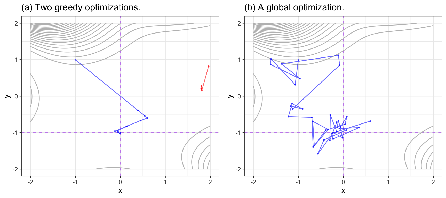
Figure 10.1 visually contrasts greedy and non-greedy search methods using the Goldstein-Price equation:
\[ \begin{align} f(x, y) &= [1+(x+y+1)^2(19-14x+3x^2-14y+6xy+3y^2)] \times \notag \\ & [30+(2x-3y)^2(18-32x+12x^2+48y-36xy+27y^2)] \notag \end{align} \]
The minimum of this function, where both \(x\) and \(y\) are between -2 and 2, is located at \(x = 0\) and \(y = -1\). The function’s outcome is relatively flat in the middle with large values along the top and lower-right edges. Panel (a) shows the results of two greedy methods that use gradient decent to find the minimum. The first starting value (in red, top right) moves along a path defined by the gradient and stalls at a local minimum. It is unable to re-evaluate the search. The second attempt, starting at \(x = -1\) and \(y = 1\), also follows a different greedy path and, after some course-corrections, finds a solution close to the best value. Each change in the path was to a new direction of immediate benefit. Panel (b) shows a global search methods called simulated annealing. This is a controlled but random approach that will be discussed in greater detail later. It generates a new candidate point using random deviations from the current point. If the new point is better, the process continues. If it is a worse solution, it may accept it with a certain probability. In this way, the global search does not always proceed in the current best direction and tends to explore a broader range of candidate values. In this particular search, a value near the optimum is determined very quickly.
Given the advantages and disadvantages of the different types of feature selection methods, how should one utilize these techniques? A good strategy which we use in practice is to start the feature selection process with one or more intrinsic methods to see what they yield. Note that it is unrealistic to expect that models using intrinsic feature selection would select the same predictor subset, especially if linear and nonlinear methods are being compared. If a non-linear intrinsic method has good predictive performance, then we could proceed to a wrapper method that is combined with a non-linear model. Similarly, if a linear intrinsic method has good predictive performance, then we could proceed to a wrapper method combined with a linear model. If multiple approaches select large predictor sets then this may imply that reducing the number of features may not be feasible.
Before proceeding, let’s examine the effect of irrelevant predictors on different types of models and how the effect changes over different scenarios.
10.3 Effect of Irrelevant Features
How much do extraneous predictors hurt a model? Predictably, that depends on the type of model, the nature of the predictors, as well as the ratio of the size of the training set to the number of predictors (a.k.a the \(p:n\) ratio). To investigate this, a simulation was used to emulate data with varying numbers of irrelevant predictors and to monitor performance. The simulation system is taken from Sapp, Laan, and Canny (2014) and consists of a nonlinear function of the 20 relevant predictors:
\[\begin{align} y = & x_1 + \sin(x_2) + \log(|x_3|) + x_4^2 + x_5x_6 + I(x_7x_8x_9 < 0) + I(x_{10} > 0) + \notag \\ & x_{11}I(x_{11} > 0) + \sqrt{|x_{12}|} +\cos(x_{13}) + 2x_{14} + |x_{15}| + I(x_{16} < -1) + \notag \\ & x_{17}I(x_{17} < -1) - 2 x_{18}- x_{19}x_{20} + \epsilon \end{align}\]
Each of these predictors was generated using independent standard normal random variables and the error was simulated as random normal with a zero mean and standard deviation of 3. To evaluate the effect of extra variables, varying numbers of random standard normal predictors (with no connection to the outcome) were added. Between 10 and 200 extra columns were appended to the original feature set. The training set size was either \(n = 500\) or \(n = 1,000\). The root mean squared error (RMSE) was used to measure the quality of the model using a large simulated test set since RMSE is a good estimate of irreducible error.
A number of models were tuned and trained for each of the simulated data sets, including linear, nonlinear, and tree/rule-based models2. The details and code for the each model can be found in a GitHub repo3 and the results are summarized below.
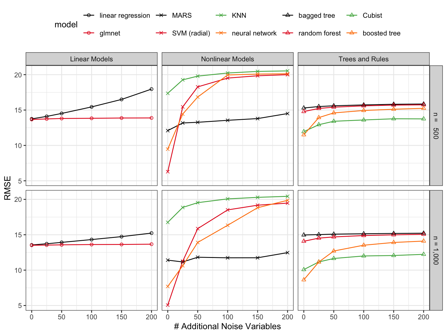
Figure 10.2 shows the results. The linear models (ordinary linear regression and the glmnet) showed mediocre performance overall. Extra predictors eroded the performance of linear regression while the lasso penalty used by the glmnet resulted in stable performance as the number of irrelevant predictors increased. The effect on linear regression was smaller as the training set size increases from 500 to 1,000. This reinforces the notation that the \(p:n\) ratio may be the underlying issue.
Nonlinear models had different trends. \(K\)-nearest neighbors had overall poor performance that was moderately impacted by the increase in \(p\). MARS performance was good and showed good resistance to noise features due to the intrinsic feature selection used by that model. Again, the effect of extra predictors was smaller with the larger training set size. Single layer neural networks and support vector machines showed the overall best performance (getting closest to the best possible RMSE of 3.0) when no extra predictors were added. However, both methods were drastically affected by the inclusion of noise predictors to the point of having some of the worst performance seen in the simulation.
For trees, random forest and bagging showed similar but mediocre performance that was not affected by the increase in \(p\). The rule-based ensemble Cubist and boosted trees faired better. However, both models showed a moderate decrease in performance as irrelevant predictors were added; boosting was more susceptible to this issue than Cubist.
These results clearly show that there are a number of models that may require a reduction of predictors to avoid a decrease in performance. Also, for models such as random forest or the glmnet, it appears that feature selection may be useful to find a smaller subset of predictors without affecting the model’s efficacy.
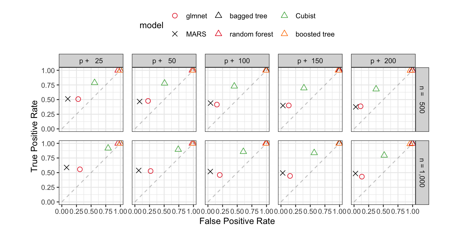
Since this is a simulation, we can also assess how models with built-in feature selection performed at finding the correct predictor subset. There are 20 relevant predictors in the data. Based on which predictors were selected, a sensitivity-like proportion can be computed that describes the rate at which the true predictors were retained in the model. Similarly, the number of irrelevant predictors that were selected gives a sense of the false positive rate (i.e., one minus specificity) of the selection procedure. Figure 10.3 shows these results using a plot similar to how ROC curves are visualized.
The three tree ensembles (bagging, random forest, and boosting) have excellent true positive rates; the truly relevant predictors are almost always retained. However, they also show poor results for irrelevant predictors by selecting many of the noise variables. This is somewhat related to the nature of the simulation where most of the predictors enter the system as smooth, continuous functions. This may be causing the tree-based models to try too hard to achieve performance by training deep trees or larger ensembles.
Cubist had a more balanced result where the true positive rate was greater than 70\(\%\). The false positive rate is around 50\(\%\) for a smaller training set size and increased when the training set was larger and less than or equal to 100 extra predictors. The overall difference between the Cubist and tree ensemble results can be explained by the factor that Cubist uses an ensemble of linear regression models that are fit on small subsets of the training set (defined by rules). The nature of the simulation system might be better served by this type of model.
Recall that the main random forest tuning parameter, \(m_{try}\), is the number of randomly selected variables that should be evaluated at each split. While this encourages diverse trees (to improve performance), it can necessitate the splitting of irrelevant predictors. Random forest often splits on the majority of the predictors (regardless of their importance) and will vastly over-select predictors. For this reason, an additional analysis might be needed to determine which predictors are truly essential based on that model’s variable importance scores. Additionally, trees in general poorly estimate the importance of highly correlated predictors. For example, adding a duplicate column that is an exact copy of another predictor will numerically dilute the importance scores generated by these models. For this reason, important predictors can have low rankings when using these models.
MARS and the glmnet also made trade-offs between sensitivity and specificity in these simulations that tended to favor specificity. These models had false positive rates under 25\(\%\) and true positive rates that were usually between 40\(\%\) and 60\(\%\).
10.4 Overfitting to Predictors and External Validation
Section 3.5 introduced a simple example of the problem of overfitting the available data during selection of model tuning parameters. The example illustrated the risk of finding tuning parameter values that over-learn the relationship between the predictors and the outcome in the training set. When models over-interpret patterns in the training set, the predictive performance suffers with new data. The solution to this problem is to evaluate the tuning parameters on a data set that is not used to estimate the model parameters (via validation or assessment sets).
An analogous problem can occur when performing feature selection. For many data sets it is possible to find a subset of predictors that has good predictive performance on the training set but has poor performance when used on a test set or other new data set. The solution to this problem is similar to the solution to the problem of overfitting: feature selection needs to be part of the resampling process.
Unfortunately, despite the need, practitioners often combine feature selection and resampling inappropriately. The most common mistake is to only conduct resampling inside of the feature selection procedure. For example, suppose that there are five predictors in a model (labeled as A though E) and that each has an associated measure of importance derived from the training set (with A being the most important and E being the least). Applying backwards selection, the first model would contain all five predictors, the second would remove the least important (E in this example), and so on. A general outline of one approach is:
\begin{algorithm} \begin{algorithmic} \STATE Rank the predictors using the training set \FOR{a feature subset of size 5 to 1} \FOR{each resample} \STATE Fit model with the feature subset on the analysis set \STATE Predict the assessment set \ENDFOR \STATE Determine the best feature subset using resampled performance \STATE Fit the best feature subset using the entire training set \ENDFOR \end{algorithmic} \end{algorithm}
There are two key problems with this procedure:
Since the feature selection is external to the resampling, resampling cannot effectively measure the impact (good or bad) of the selection process. Here, resampling is not being exposed to the variation in the selection process and therefore cannot measure its impact.
The same data are being used to measure performance and to guide the direction of the selection routine. This is analogous to fitting a model to the training set and then re-predicting the same set to measure performance. There is an obvious bias that can occur if the model is able to closely fit the training data. Some sort of out-of-sample data are required to accurately determine how well the model is doing. If the selection process results in overfitting, there are no data remaining that could possibly inform us of the problem.
As a real example of this issue, Ambroise and McLachlan (2002) reanalyzed the results of Guyon et al. (2002) where high-dimensional classification data from a RNA expression microarray were modeled. In these analyses, the number of samples was low (i.e., less than 100) while the number of predictors was high (2K to 7K). Linear support vector machines were used to fit the data and backwards elimination (a.k.a. RFE) was used for feature selection. The original analysis used leave-one-out (LOO) cross validation with the scheme outlined above. In these analyses, LOO resampling reported error rates very close to zero. However, when a set of samples were held out and only used to measure performance, the error rates were measured to be 15%–20% higher. In one case, where the \(p:n\) ratio was at its worst, Ambroise and McLachlan (2002) shows that a zero LOO error rate could sill be achieved even when the class labels were scrambled.
A better way of combining feature selection and resampling is to make feature selection a component of the modeling process. Feature selection should be incorporated the same way as preprocessing and other engineering tasks. What we mean is that that an appropriate way to perform feature selection is to do this inside of the resampling process4. Using the previous example with five predictors the algorithm for feature selection within resampling is modified to:
\begin{algorithm} \begin{algorithmic} \STATE Split data into analysis and assessment sets; \FOR{each resample} \STATE Rank the predictors using the analysis set \FOR{a feature subset of size 5 to 1} \STATE Fit model with the feature subset on the analysis set \STATE Predict the assessment set \ENDFOR \STATE Average the resampled performance for each model and feature subset size \STATE Fit the best feature subset using the entire training set \STATE Choose the model and feature subset with the best performance \STATE Fit a model with the best feature subset using the entire training set \ENDFOR \end{algorithmic} \end{algorithm}
In this procedure, the same data set are not being used to determine both the optimal subset size and the predictors within the subset. Instead different versions of the data are used for each purpose. The external resampling loop is used to decide how far down the removal path that the selection process should go. This is then used to decide the subset size that should be used in the final model on the entire training set. Basically, the subset size is treated as a tuning parameter. In addition, separate data are then used to determine the direction that the selection path should take. The direction is determined by the variable rankings computed on analysis sets (inside of resampling) or the entire training set (for the final model).
Performing feature selection within the resampling process has two notable implications. The first implication is that the process provides a more realistic estimate of predictive performance. It may be hard to conceptualize the idea that different sets of features may be selected during resampling. Recall, resampling forces the modeling process to use different data sets so that the variation in performance can be accurately measured. The results reflect different realizations of the entire modeling process. If the feature selection process is unstable, it is helpful to understand how noisy the results could be. In the end, resampling is used to measure the overall performance of the modeling process and tries to estimate what performance will be when the final model is fit to the training set with the best predictors. The second implication is an increase in computational burden5. For models that are sensitive to the choice of tuning parameters, there may be a need to retune the model when each subset is evaluated. In this case, a separate, nested resampling process is required to tune the model. In many cases, the computational costs may make the search tools practically infeasible.
In situations where the selection process is unstable, using multiple resamples is an expensive but worthwhile approach. This could happen if the data set were small, and/or if the number of features were large, or if an extreme class imbalance exists. These factors might yield different feature sets when the data are slightly changed. On the other extreme, large data sets tend to greatly reduce the risk of overfitting to the predictors during feature selection. In this case, using separate data splits for feature ranking/filtering, modeling, and evaluation can be both efficient and effective.
10.5 A Case Study
One of our recent collaborations highlights the perils of incorrectly combining feature selection and resampling. In this problem, a researcher had collected 75 samples from each of the two classes. There were approximately 10,000 predictors for each data point. The ultimate goal was to attempt to identify a subset of predictors that had the ability to classify samples into the correct response with an accuracy of at least 80%.
The researcher chose to use 70% of the data for a training set, 10-fold cross-validation for model training, and the implicit feature selection methods of the glmnet and random forest. The best cross-validation accuracy found after a broad search through the tuning parameter space of each model was just under 60%, far from the desired performance. Reducing the dimensionality of the problem might help, so principal component analysis followed by linear discriminant analysis and partial least squares discriminant analysis were tried next. Unfortunately, the cross-validation accuracy of these methods was even worse.
The researcher surmised that part of the challenge in finding a predictive subset of variables was the vast number of irrelevant predictors in the data. The logic was then to first identify and select predictors that had a univariate signal with the response. A t-test was performed for each predictors, and predictors were ranked by significance of separating the classes. The top 300 predictors were selected for modeling.
To demonstrate that this selection approach was able to identify predictors that captured the best predictors for classifying the response, the researcher performed principal component analysis on the 300 predictors and plotted the samples projected onto first two components colored by response category. This plot revealed near perfect classification between groups, and the researcher concluded that there was good evidence of predictors that could classify the samples.
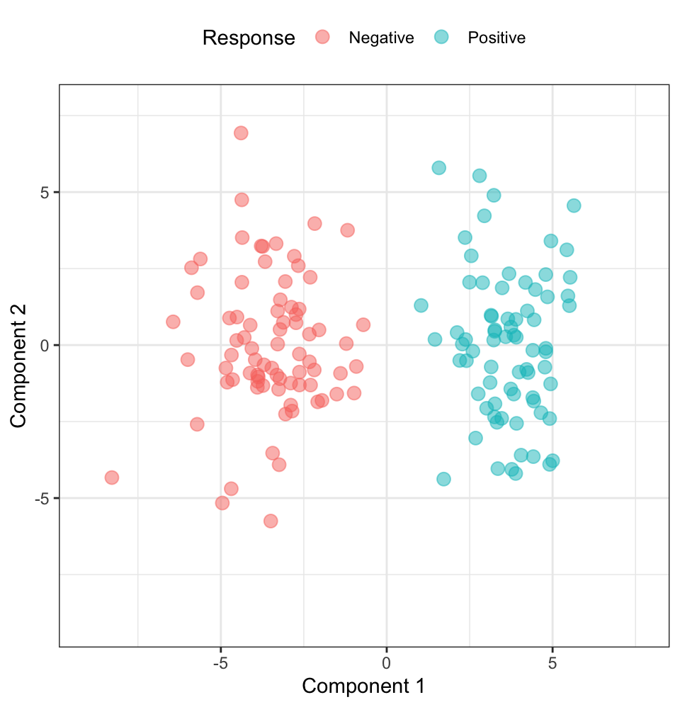
Regrettably, because feature selection was performed outside of resampling, the apparent signal that was found was simply due to random chance. In fact, the univariate feature selection process used by the researcher can be shown to produce perfect separation between two groups in completely random data. To illustrate this point we have generated a 150-by-10,000 matrix of random standard normal numbers (\(\mu = 0\) and \(\sigma = 1\)). The response was also a random selection such that 75 samples were in each class. A t-test was performed for each predictor and the top 300 predictors were selected. The plot of the samples onto the first two principal components colored by response status is displayed in Figure 10.4.
Clearly having good separation using this procedure does not imply that the selected features have the ability to predict the response. Rather, it is as likely that the apparent separation is due to random chance and an improper feature selection routine.
10.6 Next Steps
In the following chapters, the topics that were introduced here will be revisited with examples. In the next chapter, greedy selection methods will be described (such as simple filters and backwards selection). Then the subsequent chapter describes more complex (and computationally costly) approaches that are not greedy and more likely to find a better local optimum.
10.7 Computing
The website http://bit.ly/fes-selection contains R programs for reproducing these analyses.
Chapter References
Ambroise, C, and G McLachlan. 2002. “Selection Bias in Gene Extraction on the Basis of Microarray Gene-Expression Eata.” Proceedings of the National Academy of Sciences 99 (10): 6562–66.
Guyon, I, J Weston, S Barnhill, and V Vapnik. 2002. “Gene Selection for Cancer Classification Using Support Vector Machines.” Machine Learning 46 (1): 389–422.
Sapp, S, Mark J M van der Laan, and J Canny. 2014. “Subsemble: An Ensemble Method for Combining Subset-Specific Algorithm Fits.” Journal of Applied Statistics 41 (6): 1247–59.
Shmueli, G. 2010. “To Explain or to Predict?” Statistical Science 25 (3): 289–310.
An example of this was discussed in the context of simple screening in Section 7.3.↩︎
Clearly, this data set requires nonlinear models. However, the simulation is being used to look at the relative impact of irrelevant predictors (as opposed to absolute performance). For linear models, we assumed that the interaction terms \(x_5x_6\) and \(x_{19}x_{20}\) would be identified and included in the linear models.↩︎
Even if it is a single (hopefully large) validation set.↩︎
Global search methods described in Chapter 12 also exacerbate this problem.↩︎